Estimating Emissions from Sources of Air Pollution
6.2 Estimating Emissions from On-Road Mobile Sources
6.2.10 Determination of Total Driving in a Region
6.2.10.1 Introduction
One of the most difficult estimates to make in a region is the total driving that is taking place. In some urban areas, government agencies use rubber hoses across a roadway or other means to measure the vehicle kilometers traveled (VKT) on each roadway and to sum it up over the region of interest. This data often involves hundreds of roadways and is the most accurate source of total VKT. Unfortunately, many locations of interest do not have this type of data and the researcher must use other means to gather the needed information. Four methods are proposed here for making a rough estimate of total VKT.
1. The researcher can make vehicle counts themselves on a group of representative streets and extrapolate that data to the entire region of interest.
2. The researcher can determine the percentage of certain vehicle types on the street, determine the amount of driving that those vehicles carry out, and then estimate the total VKT.
3. The researcher can determine the typical daily driving of different vehicle types, the numbers of each of those vehicle types that operate on the streets each day, and then multiply the two and sum the results.
4. The researcher could use some form of aerial or satellite photography to count vehicles on different roadways and then extrapolate to the entire region of interest.
6.2.10.2 Use of Limited On-Road Vehicle for Estimating Total VKT
It is possible using videotape data, as described in Section 6.2-5, to count the vehicles that come down a roadway. It is also possible to use individuals to record data on a simple pad of paper; or the typical vehicle counting rubber hoses can be obtained or built and stretched across a roadway to detect vehicles as they pass. This is the standard way for estimating VKT in urban areas. The issue is how many roadways must be checked.
At a minimum, measurements should be made on all road types found in the region of interest. Typically roadways can be broken into three road types. These are highways, arterials, and residential streets. A highway is defined as a roadway that connects an urban area with another urban area or at a minimum crosses most of an urban area. An arterial is defined as a roadway that connects different sections of an urban area and is a prime route for traveling from one section or subsection of an urban area to another. Residential streets are the roadways that allow travel within a residential area or within a limited commercial/residential area. There are, of course, roadways that seem to fit in between the described types, but they are usually allocated to one roadway type or another. Thus, to collect roadway counts that can be extrapolated to the whole metropolitan area, counts should be made on all three types of roadways.
In the limited studies carried out by ISSRC, three roadways of each type in different parts of a city are studied. It is not recommended that a VKT study be limited to just nine roadways as described, but ISSRC studies to date have been limited to two week periods, which limit the number of roadways that can be studied. Statistics can be used to give the researcher an idea of VKT if adequate roadways have been tested. Using the student t-type test, it can be shown that the likelihood of data averaged from a statistical sample to be near the true value can be written as shown in equation 6.2.10-1.
where,
P = percentage range of values around the mean for the desired probability that the actual mean lies within the indicated range..
σ = standard deviation of the data set
A = the average value of the data set
T = a statistical constant that varies depending upon the number of samples taken and the probability that the research wants to ensure data accuracy. Some values of T are shown in table 6.2.10-2.
n = the number of samples that are taken.
Table 6.2.10-3 provides an example of a possible calculation procedure. The reliability of the data can be estimated using standard statistical technique.
Using equation 6.2.10-1, table 6.2.10-2, and table 6.2.10-3 to a 95% probability, the actual average driving on the arterials in the region will be within ±(152.8/966.7)*(4.30/√3)*100 or ±39.2% of the measured average driving. This is not a great estimate. In the case of the highway measurements, to a 95% probability the actual average driving on the highways in the region will be within ±(282.3/1466.7)*(2.57/√6)*100 or ±20.2%. This is better, but an even better estimate would be preferred. Thus, more roadways should be surveyed. For example, if 20 highways were surveyed resulting in a similar average and standard deviation as shown in table 6.2.10-3, the researcher could feel that he has a 95% probability of being within 9% of the correct average traffic count value.
Once the average vehicle counts for the different road types have been established, the length of roadways in each classification must be determined for the region of interest. Then it is a simple matter to multiply the traffic counts on each type of roadway with the total length of each type of roadway and sum then to estimate the total VKT for the region of interest.
6.2.10.3 Use of On-Road Vehicle Percentages for Estimating Total VKT
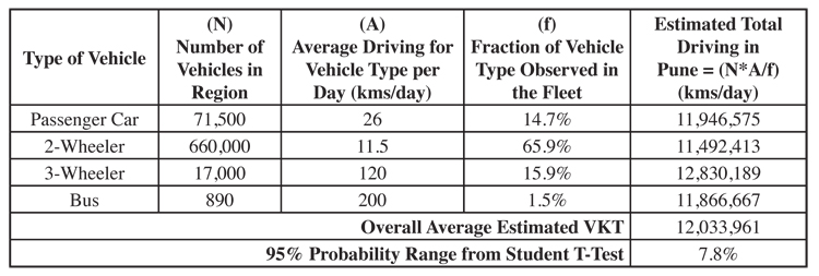
If the total VKT of a subclass of vehicles is known, and observations of the fraction of driving on a representative sample of roadways is available, then it is possible to use this information to extrapolate to the total travel of the entire fleet. For example, consider data collected in Pune, India as shown in table 6.2.10-4. This data was collected in 2003 by ISSRC and the University of California at Riverside.
In this case, estimates of total VKT per day were estimated using vehicle related parameters collected during the study. For example, the local bus company operated 890 buses keeping data on how much they were operated each day. An average public bus drove 200 kilometers per day. A video campaign determined that the public buses represented 1.5% of the vehicle traffic observed on the roadways. Thus, it was approximated that the total VKT for the city would be (890*200/0.015) or 11,866,700 kilometers per day. Similarly, it was found that there were 72,000 passenger vehicles operating in the city. A survey of vehicle odometers determined that the typical vehicle drove 24.2 kilometers per day. The roadway survey for the region determined that passenger cars make up 14.6% of the on-road fleet. This data can be used to extrapolate a total VKT of (72,000*24.2)/0.146) or 11,946,600 kilometers per day. Similar approaches were used for 2-wheel vehicles and 3-wheel vehicles resulting in an average estimated total VKT of 12,000,000 kilometers per day. While the total VKT numbers derived were not in total agreement, they produce results within 7% of the overall average.
6.2.10.4 Use of Typical Daily Driving for Estimating Total VKT
If the typical daily driving of on-road vehicles can be determined and the number of those vehicles is determined, then it is relatively straightforward to multiply the number of vehicles in each vehicle class times the average driving in that class and sum the results to estimate the total VKT. All significant classes of vehicles must be considered in making an estimate by this method. It should be warned that vehicle registration data in many cities is of very poor quality and can lead to misleading results. It should also be recalled that older vehicles tend to be operated less than newer vehicles and this has to be taken into consideration. Please see Section 6.2.5 for a discussion of these latter issues.
6.2.10.5 Use of Aerial or Satellite Photography to Make Vehicle Counts for Estimating Total VKT
A final methodology that should be mentioned is the use of aerial photography. The approach is the same as taking traffic counts using rubber hoses across roadways, individuals recording data, or video taping of traffic. In this case, aerial photographs are taken from a high enough vantage point to allow the identification of individual vehicles on the roadways and to include several kilometers of roadways in the photograph. If photographs are taken of several sections of the city at different times of the day, it is possible to actually count the vehicles on the streets at differing times of the day. Of course, the lengths of the different roadway classes must be determined in order to use the aerial data to project a region wide VKT, but it can be done by hour of the day to allow improved modeling of vehicle emissions.
One of the most difficult estimates to make in a region is the total driving that is taking place. In some urban areas, government agencies use rubber hoses across a roadway or other means to measure the vehicle kilometers traveled (VKT) on each roadway and to sum it up over the region of interest. This data often involves hundreds of roadways and is the most accurate source of total VKT. Unfortunately, many locations of interest do not have this type of data and the researcher must use other means to gather the needed information. Four methods are proposed here for making a rough estimate of total VKT.
1. The researcher can make vehicle counts themselves on a group of representative streets and extrapolate that data to the entire region of interest.
2. The researcher can determine the percentage of certain vehicle types on the street, determine the amount of driving that those vehicles carry out, and then estimate the total VKT.
3. The researcher can determine the typical daily driving of different vehicle types, the numbers of each of those vehicle types that operate on the streets each day, and then multiply the two and sum the results.
4. The researcher could use some form of aerial or satellite photography to count vehicles on different roadways and then extrapolate to the entire region of interest.
6.2.10.2 Use of Limited On-Road Vehicle for Estimating Total VKT
It is possible using videotape data, as described in Section 6.2-5, to count the vehicles that come down a roadway. It is also possible to use individuals to record data on a simple pad of paper; or the typical vehicle counting rubber hoses can be obtained or built and stretched across a roadway to detect vehicles as they pass. This is the standard way for estimating VKT in urban areas. The issue is how many roadways must be checked.
At a minimum, measurements should be made on all road types found in the region of interest. Typically roadways can be broken into three road types. These are highways, arterials, and residential streets. A highway is defined as a roadway that connects an urban area with another urban area or at a minimum crosses most of an urban area. An arterial is defined as a roadway that connects different sections of an urban area and is a prime route for traveling from one section or subsection of an urban area to another. Residential streets are the roadways that allow travel within a residential area or within a limited commercial/residential area. There are, of course, roadways that seem to fit in between the described types, but they are usually allocated to one roadway type or another. Thus, to collect roadway counts that can be extrapolated to the whole metropolitan area, counts should be made on all three types of roadways.
In the limited studies carried out by ISSRC, three roadways of each type in different parts of a city are studied. It is not recommended that a VKT study be limited to just nine roadways as described, but ISSRC studies to date have been limited to two week periods, which limit the number of roadways that can be studied. Statistics can be used to give the researcher an idea of VKT if adequate roadways have been tested. Using the student t-type test, it can be shown that the likelihood of data averaged from a statistical sample to be near the true value can be written as shown in equation 6.2.10-1.

where,
P = percentage range of values around the mean for the desired probability that the actual mean lies within the indicated range..
σ = standard deviation of the data set
A = the average value of the data set
T = a statistical constant that varies depending upon the number of samples taken and the probability that the research wants to ensure data accuracy. Some values of T are shown in table 6.2.10-2.
n = the number of samples that are taken.
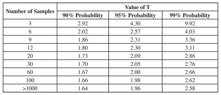
Table 6.2.10-3 provides an example of a possible calculation procedure. The reliability of the data can be estimated using standard statistical technique.
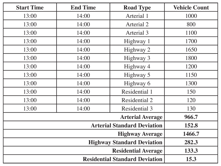
Using equation 6.2.10-1, table 6.2.10-2, and table 6.2.10-3 to a 95% probability, the actual average driving on the arterials in the region will be within ±(152.8/966.7)*(4.30/√3)*100 or ±39.2% of the measured average driving. This is not a great estimate. In the case of the highway measurements, to a 95% probability the actual average driving on the highways in the region will be within ±(282.3/1466.7)*(2.57/√6)*100 or ±20.2%. This is better, but an even better estimate would be preferred. Thus, more roadways should be surveyed. For example, if 20 highways were surveyed resulting in a similar average and standard deviation as shown in table 6.2.10-3, the researcher could feel that he has a 95% probability of being within 9% of the correct average traffic count value.
Once the average vehicle counts for the different road types have been established, the length of roadways in each classification must be determined for the region of interest. Then it is a simple matter to multiply the traffic counts on each type of roadway with the total length of each type of roadway and sum then to estimate the total VKT for the region of interest.
6.2.10.3 Use of On-Road Vehicle Percentages for Estimating Total VKT
If the total VKT of a subclass of vehicles is known, and observations of the fraction of driving on a representative sample of roadways is available, then it is possible to use this information to extrapolate to the total travel of the entire fleet. For example, consider data collected in Pune, India as shown in table 6.2.10-4. This data was collected in 2003 by ISSRC and the University of California at Riverside.
In this case, estimates of total VKT per day were estimated using vehicle related parameters collected during the study. For example, the local bus company operated 890 buses keeping data on how much they were operated each day. An average public bus drove 200 kilometers per day. A video campaign determined that the public buses represented 1.5% of the vehicle traffic observed on the roadways. Thus, it was approximated that the total VKT for the city would be (890*200/0.015) or 11,866,700 kilometers per day. Similarly, it was found that there were 72,000 passenger vehicles operating in the city. A survey of vehicle odometers determined that the typical vehicle drove 24.2 kilometers per day. The roadway survey for the region determined that passenger cars make up 14.6% of the on-road fleet. This data can be used to extrapolate a total VKT of (72,000*24.2)/0.146) or 11,946,600 kilometers per day. Similar approaches were used for 2-wheel vehicles and 3-wheel vehicles resulting in an average estimated total VKT of 12,000,000 kilometers per day. While the total VKT numbers derived were not in total agreement, they produce results within 7% of the overall average.
6.2.10.4 Use of Typical Daily Driving for Estimating Total VKT
If the typical daily driving of on-road vehicles can be determined and the number of those vehicles is determined, then it is relatively straightforward to multiply the number of vehicles in each vehicle class times the average driving in that class and sum the results to estimate the total VKT. All significant classes of vehicles must be considered in making an estimate by this method. It should be warned that vehicle registration data in many cities is of very poor quality and can lead to misleading results. It should also be recalled that older vehicles tend to be operated less than newer vehicles and this has to be taken into consideration. Please see Section 6.2.5 for a discussion of these latter issues.
6.2.10.5 Use of Aerial or Satellite Photography to Make Vehicle Counts for Estimating Total VKT
A final methodology that should be mentioned is the use of aerial photography. The approach is the same as taking traffic counts using rubber hoses across roadways, individuals recording data, or video taping of traffic. In this case, aerial photographs are taken from a high enough vantage point to allow the identification of individual vehicles on the roadways and to include several kilometers of roadways in the photograph. If photographs are taken of several sections of the city at different times of the day, it is possible to actually count the vehicles on the streets at differing times of the day. Of course, the lengths of the different roadway classes must be determined in order to use the aerial data to project a region wide VKT, but it can be done by hour of the day to allow improved modeling of vehicle emissions.