Estimating Emissions from Sources of Air Pollution
6.2 Estimating Emissions from On-Road Mobile Sources
6.2.7 Determination of Driving Patterns of On-Road Vehicles
6.2.7.1 Introduction
A critical variable in the determination of vehicle emissions is how vehicles are driven in the location of interest. The Mobile, EMFAC, and COPERT models use average road speeds to establish driving patterns. The MOVES, IVE, and CMEM models are more flexible in incorporating vehicle operations into the model and do not need to rely on a set group of cycles to estimate emissions. Instead, actual driving data is used to predict emissions, and it relies on more specific driving parameterization than simply average speed. In this case, it is not always a simple task to obtain the needed driving pattern information. It is possible to interface to vehicle computer systems and record how vehicles drive. However, the interfaces to vehicle computer systems are not always the same and the monitoring equipment can be expensive. An alternate approach is to attach a monitor, such as a global position system (GPS) to a vehicle to record the vehicle speeds. In order to obtain the data needed for the MOVES, IVE, Handbook, and CMEM models, at least second by second speed and altitude data must be recorded. GPS units are available that record data several times per second; however, these have not been found to significantly improve the data over second by second measurements.
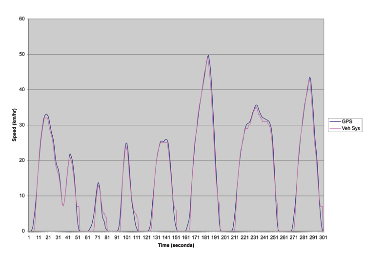
Two options have been used in ISSRC studies to record speeds on a second by second bases. One is an optical sensor that attaches to the bumper of a vehicle that determines the vehicle speed. The other is the use of recording Global Positioning Satellite (GPS) systems. Overall, the optical sensor has proven to be the more reliable, but the GPS is also very accurate, smaller, easier to use, and cheaper. Thus, GPS is the most common approach to establishing roadway driving patterns and average speeds. Figure 6.2.7-1 compares results from a recording GPS unit with driving speeds determined by a vehicle speed measurement system.
As can be seen in figure 6.2.7-1, the overall agreement between the two measurement systems is very good. The main differences occur at the lower speeds, which are not as important for vehicle emission determination.
There is a problem with the use of GPS that must be taken into consideration when analyzing GPS data. A GPS unit can momentarily loose contact with the satellite systems that allow it to compute speeds and location. This can be caused by trees, buildings or it may sometimes occur for no discernable reason. When these events happen, the GPS unit sometimes continues to report the old speed until the unit resumes proper operation or the speeds reported go to zero. In cases where the speed goes to zero, a large vehicle deceleration and then acceleration is recorded. Similarly in the case where the GPS unit simply maintains its prior speed, when the unit subsequently corrects itself, the unit can record a significant acceleration or deceleration. These erroneous accelerations and decelerations can result in vehicle power demand calculations that are very high positive or negative. Because they are so rare, they do not tend to influence average speeds unless there are significant losses of data. In the case of the need for second by second speeds, the GPS data must be screened for these anomalous events before it is processed. This screening is not always easy. An initial approach is to flag all large accelerations and decelerations and to review the data manually. Screening macros have also been developed by researchers using Excel and other programs to help find these anomalous events.
The GPS can also provide altitude information, which theoretically can be used to determine road grade information for the cases of significant hills. However, great care is needed in using the data for this purpose. The GPS altitude data drifts around considerably more than does the speed data. Thus, ever more care must be taken before using GPS altitude data to estimate road grades. It is best to develop some sort of curve fitting program and to collect multiple runs of GPS altitude data over the route of interest to use for this purpose.
6.2.7.2 Vehicle Specific Power
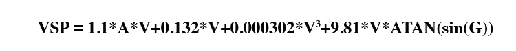
An important vehicle parameter used by the USEPA MOVES model and the IVE model is vehicle specific power (VSP). VSP is the power per unit weight involved in the vehicle movement. Equation 6.2.7-2 presents the calculation process for VSP, which was originally developed by Jimenez-Palacios (1999).
Where,
VSP = vehicle specific power (kilowatts/ton)
V = vehicle speed (m/s)
A = vehicle acceleration (m/s/s)
G = Road grade in meters elevation change per meter of road distance (radians)
The IVE model adds an air conditioning load component to equation 6.2.7-2 when determining engine load for estimating emissions.
The term (1.1*A*V) represents the kinetic power demand on the vehicle as it accelerates or decelerates. The term (0.132*V) represents the engine friction and wheel friction power demand. The term (0.000302*V3) represents the power demand due to air friction. The term V*(ATAN(sin(G))) represents the power demand due to the road slope. VSP can be positive or negative depending upon the acceleration and the road slope.
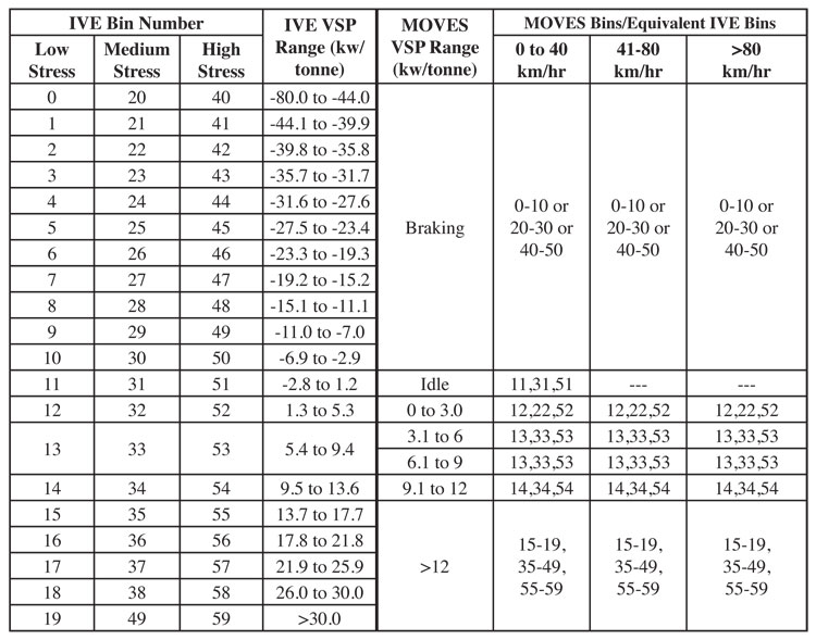
In order to make calculations, the MOVES model breaks the VSP into 17 bins. The IVE model breaks the VSP bins into 60 bins. The MOVES model uses an additional classification of vehicle speed while the IVE model uses an additional classification called Stress. Table 6.2.7-3 compares the bin definitions for the MOVES and IVE model bins in terms of VSP. Some bin definitions do not directly translate between the IVE and MOVES model. An attempt has been made to align them as well as possible.
The engine Stress term referred to in the IVE model relates to the engine rpm and the time that the vehicle has been operating at a higher VSP level. The higher the rpm and/or the higher the VSP levels for 20 seconds before an event, the higher the Stress level and thus the higher emissions produced by the engine. The engine stress category is based on the formula:
Engine Stress (unitless) = RPMIndex + (0.08 ton/kW)*PreaveragePower
where
PreaveragePower = Average(VSPt=-1sec to –21 sec) (kW/ton)
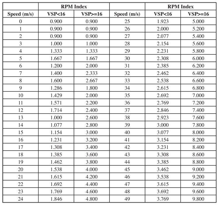
RPMIndex = is associated with the expected rpm of the vehicle engine although it is not intended to be an exact indication of the engine rpm since this will vary with the vehicle type. Table 6.2.7-4 indicates the RPMIndex based on the vehicle speed (m/s) and VSP demand on the vehicle at the time of calculation.
A vehicle is classified as in Stress category 1 if the calculated Stress value is between -1.60 and 3.10, Stress category 2 if the calculated Stress value is between 3.11 and 7.80, Stress category 3 if the calculated Stress value is greater than 7.80.
Based on studies to date almost all driving is in Stress category 1 and studies of engine stress in developing countries have found no driving in Stress category 3. Only measurements of freeway driving in the United States have found driving in Stress category 3.
In most situations, vehicle speeds are measured second by second and thus VSP is calculated second by second. Software can be downloaded from the ISSRC web site (http://www.issrc.org/ive) to take second by second GPS data and divide it into the 60 IVE VSP and Stress Bins.
It is possible to place GPS or other second by second speed recording equipment on a vehicle for a 24-hour period and record the movements of the vehicle. In the case of passenger vehicles, if this is done for more than 50 vehicles that are selected from all parts of the area of interest, the researcher should have a good set of data to establish local driving patterns. Trucks, buses and motorcycles can also be tested with similar equipment and a similar approach to establish their driving patterns.
Because of the cost of the GPS equipment, this approach, though viable and maybe even preferred, is not the approach typically selected for passenger vehicles. Instead, three tracking vehicles are often outfitted with GPS equipment and are operated on specified routes following the normal traffic from early morning until late evening to collect the needed data. Usually, the area being studied is divided into three representative regions and a highway, arterial, and residential street are selected in each region. The vehicles are then operated on each of the nine streets for each hour of the day from early morning until late evening to establish hour by hour driving patterns. With this approach, the driving patterns can be established for a city in a two week period. This is not to say that measuring more roadways and more regions of the city would not be better—it is better. However, this approach can be used as the lowest cost way to get driving pattern data for a city in a relatively short period of time.
Buses and trucks are typically treated differently from passenger vehicles. In the case of buses, bus riders can be provided with portable GPS equipment, and they can be assigned bus routes to ride. In a matter of two weeks, three riders can cover adequate bus routes at most hours of the day to establish the bus driving patterns by hour of the day. It is common to equip a truck with GPS equipment for 24-hours and to have that truck go through its normal work route. It is desirable to measure at least 25 trucks, which can be accomplished in a two week period with two recording GPS units.
Figure 6.2.7-5 illustrates the IVE bin distribution patterns measured in Nairobi, Santiago, and Sao Paulo for passenger vehicles using the tracking vehicle approach.
As can be seen in figure 6.2.7-5, there are differences between the driving patterns that were measured in the three cities, but there are similarities as well.
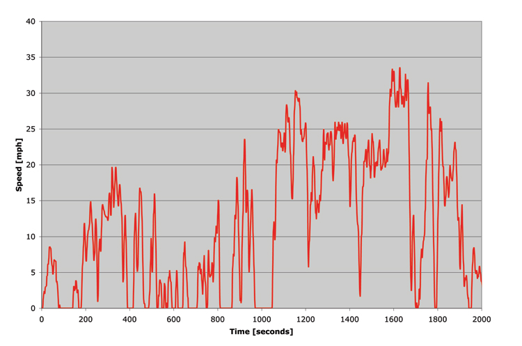
Figure 6.2.7-6 illustrates the second by second speeds of a student riding on a bus to collect bus driving pattern information.
Bus driving patterns involve numerous stops as can be seen in figure 6.2.7-6. These many stops and subsequent accelerations have a significant impact on the emissions released from these buses.
In summary, the most common method of developing driving pattern data is to use GPS equipment that stores speed, location, altitude, and satellite number on a second by second basis. This data can then be turned into an average driving pattern for use in a CMEM type model or it can be binned by vehicle specific speed (VSP) to use in an IVE or MOVES type models. GPS data sets can contain erroneous data points and care must be taken to filter out these errors.
A critical variable in the determination of vehicle emissions is how vehicles are driven in the location of interest. The Mobile, EMFAC, and COPERT models use average road speeds to establish driving patterns. The MOVES, IVE, and CMEM models are more flexible in incorporating vehicle operations into the model and do not need to rely on a set group of cycles to estimate emissions. Instead, actual driving data is used to predict emissions, and it relies on more specific driving parameterization than simply average speed. In this case, it is not always a simple task to obtain the needed driving pattern information. It is possible to interface to vehicle computer systems and record how vehicles drive. However, the interfaces to vehicle computer systems are not always the same and the monitoring equipment can be expensive. An alternate approach is to attach a monitor, such as a global position system (GPS) to a vehicle to record the vehicle speeds. In order to obtain the data needed for the MOVES, IVE, Handbook, and CMEM models, at least second by second speed and altitude data must be recorded. GPS units are available that record data several times per second; however, these have not been found to significantly improve the data over second by second measurements.
Two options have been used in ISSRC studies to record speeds on a second by second bases. One is an optical sensor that attaches to the bumper of a vehicle that determines the vehicle speed. The other is the use of recording Global Positioning Satellite (GPS) systems. Overall, the optical sensor has proven to be the more reliable, but the GPS is also very accurate, smaller, easier to use, and cheaper. Thus, GPS is the most common approach to establishing roadway driving patterns and average speeds. Figure 6.2.7-1 compares results from a recording GPS unit with driving speeds determined by a vehicle speed measurement system.
As can be seen in figure 6.2.7-1, the overall agreement between the two measurement systems is very good. The main differences occur at the lower speeds, which are not as important for vehicle emission determination.
There is a problem with the use of GPS that must be taken into consideration when analyzing GPS data. A GPS unit can momentarily loose contact with the satellite systems that allow it to compute speeds and location. This can be caused by trees, buildings or it may sometimes occur for no discernable reason. When these events happen, the GPS unit sometimes continues to report the old speed until the unit resumes proper operation or the speeds reported go to zero. In cases where the speed goes to zero, a large vehicle deceleration and then acceleration is recorded. Similarly in the case where the GPS unit simply maintains its prior speed, when the unit subsequently corrects itself, the unit can record a significant acceleration or deceleration. These erroneous accelerations and decelerations can result in vehicle power demand calculations that are very high positive or negative. Because they are so rare, they do not tend to influence average speeds unless there are significant losses of data. In the case of the need for second by second speeds, the GPS data must be screened for these anomalous events before it is processed. This screening is not always easy. An initial approach is to flag all large accelerations and decelerations and to review the data manually. Screening macros have also been developed by researchers using Excel and other programs to help find these anomalous events.
The GPS can also provide altitude information, which theoretically can be used to determine road grade information for the cases of significant hills. However, great care is needed in using the data for this purpose. The GPS altitude data drifts around considerably more than does the speed data. Thus, ever more care must be taken before using GPS altitude data to estimate road grades. It is best to develop some sort of curve fitting program and to collect multiple runs of GPS altitude data over the route of interest to use for this purpose.
6.2.7.2 Vehicle Specific Power
An important vehicle parameter used by the USEPA MOVES model and the IVE model is vehicle specific power (VSP). VSP is the power per unit weight involved in the vehicle movement. Equation 6.2.7-2 presents the calculation process for VSP, which was originally developed by Jimenez-Palacios (1999).
Where,
VSP = vehicle specific power (kilowatts/ton)
V = vehicle speed (m/s)
A = vehicle acceleration (m/s/s)
G = Road grade in meters elevation change per meter of road distance (radians)
The IVE model adds an air conditioning load component to equation 6.2.7-2 when determining engine load for estimating emissions.
The term (1.1*A*V) represents the kinetic power demand on the vehicle as it accelerates or decelerates. The term (0.132*V) represents the engine friction and wheel friction power demand. The term (0.000302*V3) represents the power demand due to air friction. The term V*(ATAN(sin(G))) represents the power demand due to the road slope. VSP can be positive or negative depending upon the acceleration and the road slope.
In order to make calculations, the MOVES model breaks the VSP into 17 bins. The IVE model breaks the VSP bins into 60 bins. The MOVES model uses an additional classification of vehicle speed while the IVE model uses an additional classification called Stress. Table 6.2.7-3 compares the bin definitions for the MOVES and IVE model bins in terms of VSP. Some bin definitions do not directly translate between the IVE and MOVES model. An attempt has been made to align them as well as possible.
The engine Stress term referred to in the IVE model relates to the engine rpm and the time that the vehicle has been operating at a higher VSP level. The higher the rpm and/or the higher the VSP levels for 20 seconds before an event, the higher the Stress level and thus the higher emissions produced by the engine. The engine stress category is based on the formula:
Engine Stress (unitless) = RPMIndex + (0.08 ton/kW)*PreaveragePower
where
PreaveragePower = Average(VSPt=-1sec to –21 sec) (kW/ton)
RPMIndex = is associated with the expected rpm of the vehicle engine although it is not intended to be an exact indication of the engine rpm since this will vary with the vehicle type. Table 6.2.7-4 indicates the RPMIndex based on the vehicle speed (m/s) and VSP demand on the vehicle at the time of calculation.
A vehicle is classified as in Stress category 1 if the calculated Stress value is between -1.60 and 3.10, Stress category 2 if the calculated Stress value is between 3.11 and 7.80, Stress category 3 if the calculated Stress value is greater than 7.80.
Based on studies to date almost all driving is in Stress category 1 and studies of engine stress in developing countries have found no driving in Stress category 3. Only measurements of freeway driving in the United States have found driving in Stress category 3.
In most situations, vehicle speeds are measured second by second and thus VSP is calculated second by second. Software can be downloaded from the ISSRC web site (http://www.issrc.org/ive) to take second by second GPS data and divide it into the 60 IVE VSP and Stress Bins.
It is possible to place GPS or other second by second speed recording equipment on a vehicle for a 24-hour period and record the movements of the vehicle. In the case of passenger vehicles, if this is done for more than 50 vehicles that are selected from all parts of the area of interest, the researcher should have a good set of data to establish local driving patterns. Trucks, buses and motorcycles can also be tested with similar equipment and a similar approach to establish their driving patterns.
Because of the cost of the GPS equipment, this approach, though viable and maybe even preferred, is not the approach typically selected for passenger vehicles. Instead, three tracking vehicles are often outfitted with GPS equipment and are operated on specified routes following the normal traffic from early morning until late evening to collect the needed data. Usually, the area being studied is divided into three representative regions and a highway, arterial, and residential street are selected in each region. The vehicles are then operated on each of the nine streets for each hour of the day from early morning until late evening to establish hour by hour driving patterns. With this approach, the driving patterns can be established for a city in a two week period. This is not to say that measuring more roadways and more regions of the city would not be better—it is better. However, this approach can be used as the lowest cost way to get driving pattern data for a city in a relatively short period of time.
Buses and trucks are typically treated differently from passenger vehicles. In the case of buses, bus riders can be provided with portable GPS equipment, and they can be assigned bus routes to ride. In a matter of two weeks, three riders can cover adequate bus routes at most hours of the day to establish the bus driving patterns by hour of the day. It is common to equip a truck with GPS equipment for 24-hours and to have that truck go through its normal work route. It is desirable to measure at least 25 trucks, which can be accomplished in a two week period with two recording GPS units.
Figure 6.2.7-5 illustrates the IVE bin distribution patterns measured in Nairobi, Santiago, and Sao Paulo for passenger vehicles using the tracking vehicle approach.
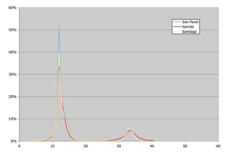
As can be seen in figure 6.2.7-5, there are differences between the driving patterns that were measured in the three cities, but there are similarities as well.
Figure 6.2.7-6 illustrates the second by second speeds of a student riding on a bus to collect bus driving pattern information.
Bus driving patterns involve numerous stops as can be seen in figure 6.2.7-6. These many stops and subsequent accelerations have a significant impact on the emissions released from these buses.
In summary, the most common method of developing driving pattern data is to use GPS equipment that stores speed, location, altitude, and satellite number on a second by second basis. This data can then be turned into an average driving pattern for use in a CMEM type model or it can be binned by vehicle specific speed (VSP) to use in an IVE or MOVES type models. GPS data sets can contain erroneous data points and care must be taken to filter out these errors.