Estimating Emissions from Sources of Air Pollution
6.2 Estimating Emissions from On-Road Mobile Sources
6.2.2 Key Emission Related Parameters and the Use of Emission Factors
6.2.2.1 Defining the Key Emission Related Parameters
Depending upon the size of the urban area under consideration, there will typically be several hundred thousand to millions of on-road vehicles operating within the confines of the urbanized area. Some of these vehicles will be old, some will be new, some will be for passengers and some will be for transporting goods. The area of interest will also typically include thousands of miles of roadways with the various roadways serving different functions. In order to make emission estimates for an on-road vehicle fleet, it must be understood how different vehicle parameters impact vehicle emissions.
Based on the discussions in the previous section it is clear that several vehicle fuel and engine parameters must be understood in order to develop an adequate understanding of the vehicle fleet. Once the vehicle fleet is categorized, then an understanding must be developed of the amount and type of driving in the area of interest. Altitude, temperature, and even humidity can also effect emissions. The fleet information and vehicle operation information can be divided and treated as separate issues for making vehicle emission estimates.
6.2.2.2 Defining Fleet Information
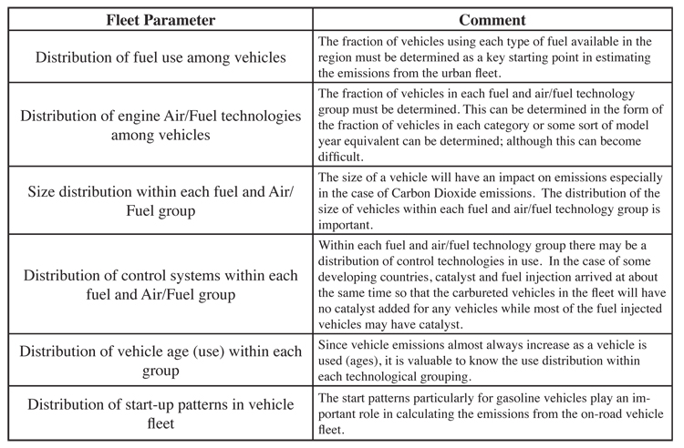
Table 6.2.2-1 describes the key components of the on-road vehicle fleet that must be understood in order to appropriately estimate the emissions from a fleet.
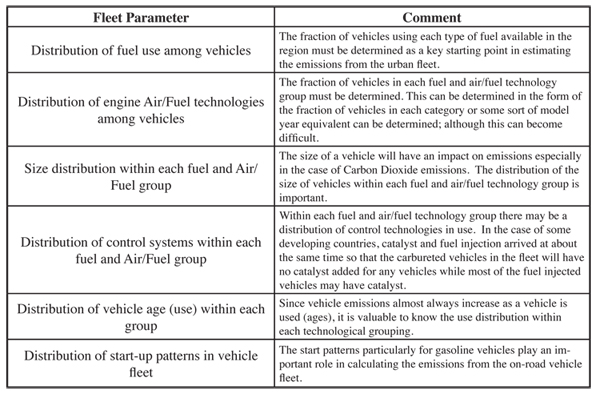
When fractions are referred to in table 6.2.2-1, it should be understood that the fraction that is ultimately desired is the dynamic fleet information, referring to the fraction of on-the road driving that each technology group carries out. This is typically different from the fraction of the static population that exists in the overall fleet. Old vehicles are operated less than new vehicles in urban and rural fleets. Thus, new vehicles typically contribute more on-road driving per vehicle than do the old vehicles and this must be accounted for in determining the dynamic fleet distributions. This is discussed further in the section on the determination of fleet technology distributions.
Since it is impossible to compile an inventory that estimates the emissions from every vehicle in the fleet, vehicles with similar emissions characteristics are grouped together to make measurements and calculations manageable. Significant research has been conducted on the most meaningful way to categorize the vehicles for emissions estimates. For example, it was found in research to develop the IVE model (discussed later) that vehicle size was not a major determiner of emissions other than for CO2 emissions. Other parameters such as vehicle age (or total use) have a more significant impact on most pollutants (i.e. a vehicle typically pollutes more as it ages). In any case, each vehicle’s technology related parameters can have some effect that should be considered. To address vehicle size and overall use, some models use groupings or binning of age or use groups. In the case of the IVE model, three vehicle size groupings are used along with three use groups. Other models use linear calculations from overall weight or total use to express emission changes. As is the case for the IVE model, if use and size are broken into three groups each, then this categorization process will produce nine emission analysis groups (often called ‘bins’) for each fuel and air/fuel technology group.
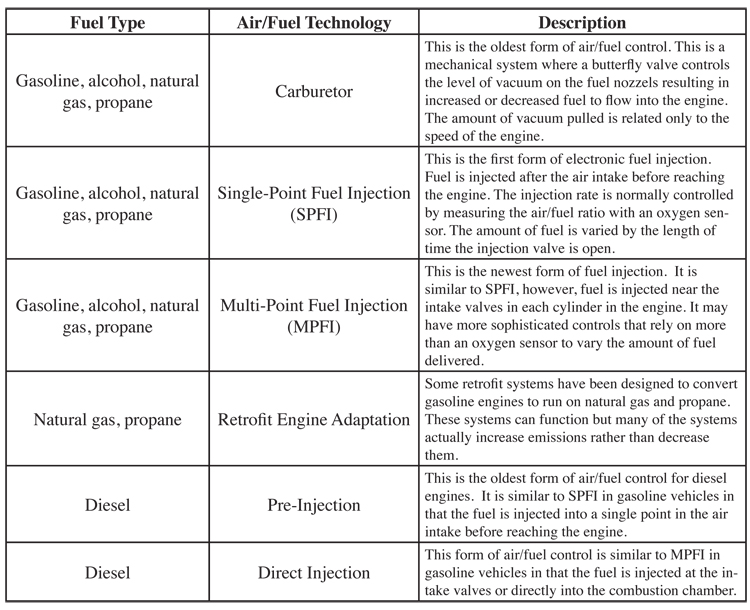
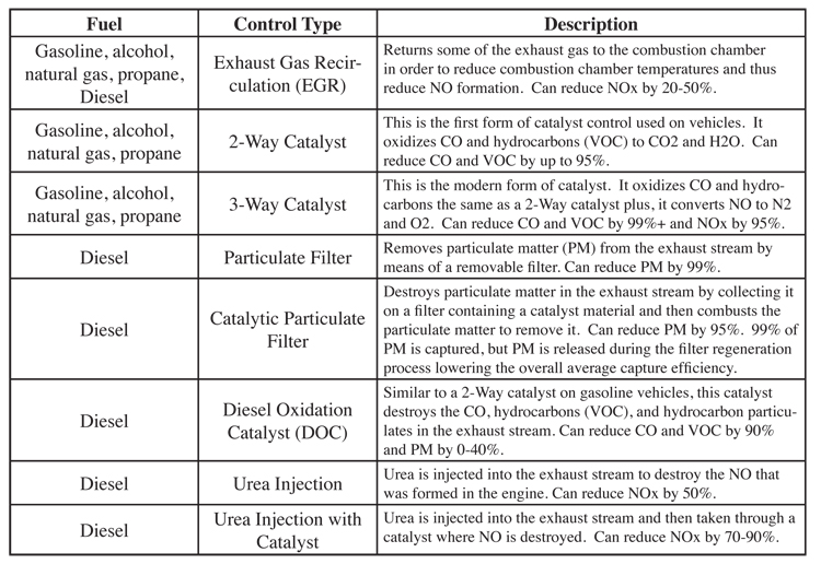
Referring to tables 6.2.2-2 and 6.2.2-3 there are five major fuel types in use today in most locations. Within each fuel type there are two to four air/fuel technologies. Within each fuel and air/fuel technology group there are about five to eight control options. This leads to the potential definition of up to 5X4X8 technology categories or about 160 technology groups. Combining this with the 9 size/use groupings discussed in the previous paragraph, then there are 1440 potential vehicle technology classifications to be considered in a given urban area.
Typically, however, all of the potential categories will not appear in a single urban fleet. Even if it did, it is easily possible to manage 1440 vehicle categories on a single Excel workbook or similar data base system. It does become a little bit overwhelming if each technology could use significantly different grades of fuel in an urban area, but all vehicles within a given urban fleet are typically exposed to the same fuel grades within their respective fuel types. If this is not the case, then further breakdowns must be carried out to handle the various fuel group categories.
It is also possible to use model year as a surrogate for vehicle technology, use, and size. In this approach, vehicles are broken into the major fuel categories found in a region of interest and an emission estimate is made for the vehicles of each fuel type for each model year. The advantage to this approach is that allowing for five major fuel types and fifteen model years there are only 75 vehicle categories to track. The negative to this approach is that a vehicle emission rate for each of the 75 vehicle categories must be developed. Since most developing countries have little or no emission measurements, it is not possible to establish appropriate emission rates for each of the 75 fuel type/year categories. In the case of the use of technology classifications as opposed to model year classifications, it can be assumed to a first approximation that vehicles of similar technology operating in different countries emit similarly. Work by ISSRC has determined that this is not totally true, but for gross approximations, it is a worthwhile beginning assumption. To be clear, ISSRC is the acronym for the International Sustainable Systems Research Center. Information concerning ISSRC activities and reports can be found at http://www.issrc.org.
A hybrid of the technology and model year approach can be used. In this case, the technology distribution for each model year for the location of interest is determined and an emission rate is calculated for each model year by multiplying the fraction of vehicles in each technology class by the emission factor for that technology class. However, this does not reduce the overall calculations that must be made since the same amount of calculations must be carried out to establish the model year emission rate for each model year as would have been required by using an overall technology breakdown.
6.2.2.3 Determining Vehicle Operation using Velocity Profiles
As discussed earlier, the manner in which vehicles operate, known as the vehicle operation information, impacts emissions significantly. This includes vehicle speed, acceleration, braking, and so forth, as well as how often they are started and how long they have soaked. Thus to evaluate emissions from a vehicle fleet, the driving and start patterns of vehicles are an important consideration. Actual driving patterns and start patterns vary throughout the day creating a complex situation for evaluating vehicle emissions.
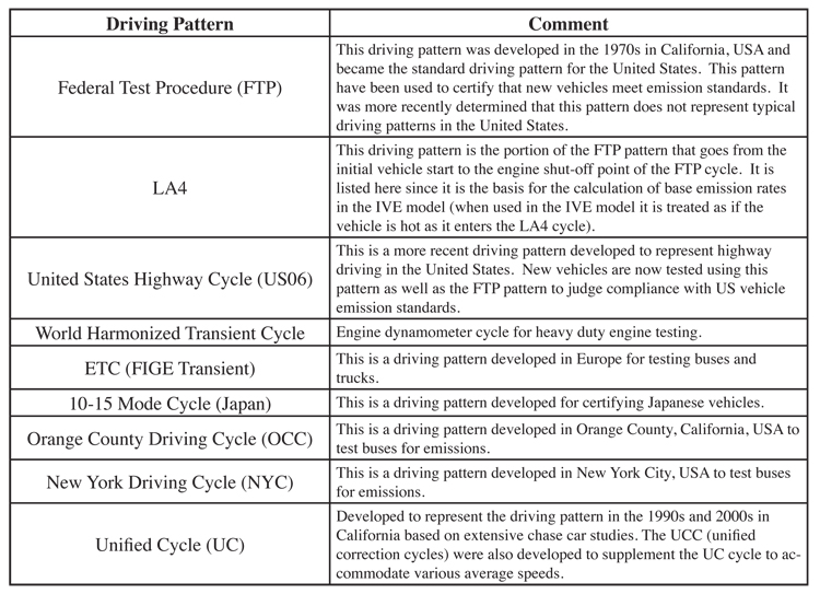
Historically, a standardized driving cycle or cycles was developed to use for measuring and predicting emissions from vehicles. There are two important reasons to determine a standardized cycle to relate emissions to. The first is to have a common measure for determining emissions in the certification or inspection process, and for comparing emissions between vehicles and vehicles as they age. The second reason is to determine the emissions that are occurring during real-world operation to be able to calculate the emissions inventory for the vehicle. Originally, the same cycle was used for both purposes. However, as the understanding of the complexity and importance of real-world driving has improved over the years, it became clear that these original cycles were inadequate and could severely underestimate emissions from real-world operation. In the United States, the first driving cycle developed is known as the Federal Test Procedure (FTP), and it was assumed that all drivers in all cities, on average, operated their vehicles consistent with this driving pattern. It was found, of course, that this is not the case and in actuality, much higher velocities and accelerations that drastically affect emissions occur on the roadways. At that time, however, vehicle dynamometers used to conduct these tests had limitations on the speed and accelerations where they could be operated. Since then the improved driving cycles, such as the supplemental FTP, the UC, and other cycles have become more commonly used for emissions inventory calculations. Other countries have developed or are developing their own driving patterns as well. A discussion of various U.S. related driving cycles can be found on the U.S. EPA web site at http://www.epa.gov/nvfel/testing/dynamometer.htm. Also, the website http://www.dieselnet.com/standards/cycles/ provides useful information related to standard driving cycles from many parts of the world. Table 6.2.2-4 presents some examples of the driving cycles in use today.
Although the FTP cycle does not accurately reflect real-world driving in many locations (including the US), it is very useful and very often used as a starting point, or base emission factor, since there is such a vast database of vehicles tested on this standardized cycle. It is common for other cycles or corrections to be applied to the base emission factor to represent changes in emissions from vehicle operation that deviates from the FTP cycle. Figure 6.2.2-5 graphs the velocity profile of the FTP driving pattern. Emissions for the FTP cycle are traditionally collected in three bags. Bag 1 begins with a cold start (18-hour soak time) and continues for approximately 505 seconds (sometimes called a ‘cold 505’). Bag 2 immediately follows Bag 1 and represents hot running stabilized emissions and lasts 867 seconds, when the engine is turned off. In the traditional FTP cycle, there is a 10 minute engine soak period where the engine remains off, then the vehicle is started while the engine is still ‘hot’ and the same driving trace conducted in the first 505 seconds is repeated. Bag 3 is sometimes called ‘hot 505’ because it contains this hot start. (A ‘hot’ start is defined as when the engine is only soaked for 10 minutes). Sometimes, a Bag 4 follows immediately after the test without turning off the engine. Bag 4 is a repeat again of the first 505 seconds in Bag1/3 except with no start at all and with a fully warmed up engine, and so it is sometimes called a ‘running 505’. So, Bags 1,3, and 4 are exactly the same driving pattern but the type of start condition is varied. It is therefore possible to know the exact emissions from an engine start by subtracting one bag from another. For example, Bag 1-Bag 4 (Cold 505- Running 505) is equal to a cold start. Similarly, Bag 3- Bag 4 (Hot 505- Running 505) gives you the hot start emissions from that particular vehicle. Often times, Bag 3-Bag 4 is close or sometimes below zero, indicating that hot start emissions are negligible over the noise of the testing instrument variability (also meaning that Bag 3 ≅ Bag 4). So, many times, especially when Bag 4 is not collected, a cold start can be estimated by Bag 3-Bag 1.
The portion of the FTP pattern in 6.2.2-5 that is considered the LA4 pattern is colored pink. This includes emissions collected in Bag 1 or Bag 3 followed by Bag 2 of the FTP cycle. A ‘cold start trip, or cold LA4, is using Bags 1 and 2, and a ‘hot’ LA4, or ‘hot start trip’ uses Bag 3 instead of Bag 1. The distance covered in Bag 1/3 is 3.59 miles and 3.91 miles for Bag 2. The overall weighted emissions of an FTP are reported in grams/mile and can be calculated as .206*Bag1 emissions/3.59 miles + .521*Bag 2 emissions/3.91 + .273*Bag 3 emissions/3.59 miles.
Since the introduction of Global Positioning Satellite Units (GPS), which can collect second by second data quickly and accurately over long periods of time, many areas are using this data to collect and design a set of representative cycles for all of the different road types and congestion situations in the areas. These are sometimes called ‘facility cycles’ by the US EPA, which has 14 different cycles to represent the speed and acceleration profile at different roadway types and levels of congestion. This is used in the newest version of the MOBILE model. California uses a set of Unified Correction Cycles to model similar effects of roadway conditions. Germany has developed a comprehensive set of 43 driving cycles from a large GPS data set.
All of the cycles developed in each area are different, however, they all are velocity profiles and they are all classified by road type. At a minimum, roadways are often classified into one of four classes:
"1. Residential Streets - Roads that carry vehicles into and through residential areas, typically exhibiting lower speeds, many stops, and/or speed bumps."
2. Arterials - Roads that connect one part of a city to another, usually with slow to moderate speeds, with some stops or stop lights.
3. Highways- Roads that connect one city to another city or cross a city, with minimal stops.
4. Freeways - Limited access roads for moving from city to city or across a city, usually with on and off-ramps and no stops.
Freeways are highly developed in the United States and parts of Europe. They are less prevalent in many developing countries. It is common to combine highways and freeways into a single road category usually referred to as Highways resulting in three categories of roadways. It also goes, almost without saying, that some residential streets operate similarly to arterials and some arterials operate similarly to highways. However, for the sake of simplicity, the three to four categories of streets as outlined above are normally used to carry out air pollution and other road related studies in urban areas.
Based on studies carried out by ISSRC in various countries around the world, the dominant number of road kilometers in an urban area is on residential streets by a three to one margin compared to arterials and highways combined. Arterials are second in total length, and highways are the least. ISSRC has also cataloged vehicle driving patterns by road type and by hour of the day for a number of cities around the world in order to understand how driving varies by road class and to improve emission estimates.
6.2.2.4 Moving beyond Static Velocity & Acceleration Profiles to Estimate Emissions Effects of Vehicle Operation
Many of the methods described in previous paragraphs use a type of velocity profile correction to model the effect of vehicle operations on emissions. This means that if a modeler would like to estimate emissions on the freeway, he would measure (or assume) the average velocity on that roadway and select a cycle that has similar average velocities. However, there are inherent problems with this approach, since the average velocity of a cycle is a poor indicator of emissions over that cycle. A much better indicator is combining velocity with acceleration. This is done in a modal emissions approach that defines an emission rate or correction for various operating modes, such as idle, cruise, and acceleration and deceleration. However, this is still a ‘static’ approach and cannot take into consideration road grade, use of accessory power consumption or other time-dependent factors such as catalyst loading or delayed responses.
Even more recently, a different, more accurate method of estimating emissions from vehicles is being used in the US and Europe that does not rely on a specific velocity-based cycle, rather a set of operational conditions that can be described using vehicle specific power. This method of characterizing vehicle operation can take into consideration dynamic factors and other considerations that have an effect on fuel use and emissions output, such as road grade, using the air conditioner, etc.
6.2.2.5 Fuel Quality
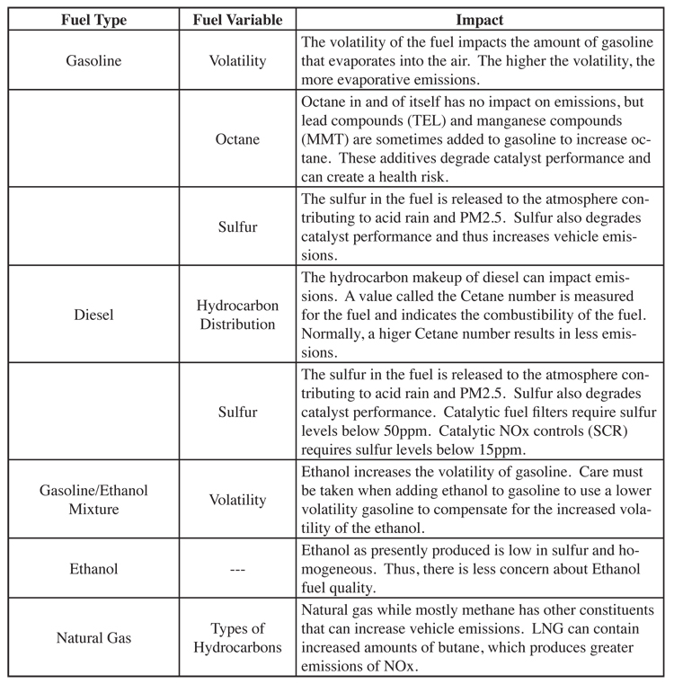
As discussed in subsection 6.2.1, fuel type and quality can have significant impacts on vehicle emissions. The most important considerations related to fuel quality are summarized in table 6.2.2-6. Most emission factors for vehicles are based on standard fuels. When estimating emissions, adjustments should be made for the cases where fuel quality results in more or less emissions than the standard fuels. Most vehicle emission models allow for some adjustment to the model calculations based on fuel quality.
6.2.2.6 Start Emissions and Start Patterns
In order to make a vehicle start easier, more fuel is normally supplied to the engine. This causes the air/fuel mixture to become richer which makes the vehicle start easier, especially in cold weather. However, this procedure also increases the emissions from the vehicle until the air/fuel ratio is returned to the normal rate. Vehicles manufactured in the United States before 1960 often had a manual adjustment for the air/fuel mixture called a “choke”, which would richen the mixture when pulled and then was manually shut off once the vehicle was warmed up. Modern vehicles handle this adjustment automatically so that the driver is normally unaware that such an adjustment is taking place. These extra emissions that occur as the vehicle is started and warmed up are referred to as start emissions. With the addition of catalysts to vehicles, the emissions associated with a vehicle start compared to normal operations increased further since the catalyst is ineffective until it is warmed up. Thus, an important emissions concern with respect to vehicles is the start emissions associated with the vehicle. Catalyst controlled vehicles tend to have relatively larger start emissions compared to non-catalyst controlled vehicles.
Start emissions are defined as the emissions in excess of normal warm vehicle emissions that occur during the first few minutes of vehicle operation. A vehicle that has been operated so that the engine and catalyst are at least somewhat warm will have less start emissions than a vehicle that has sat for a long time and the engine and catalyst are at ambient temperatures. Thus, there are different start emissions associated with a vehicle that has stopped for only a few minutes and then re-started compared to a vehicle that has not operated for 12 or more hours. The time that a vehicle is not operated is referred to as the “soak” period. The start emissions then vary with the soak period from almost zero with a soak period of less than 15 minutes to the maximum amount after about twelve hours of non-operation soak.
In order to estimate start emissions associated with a single vehicle, one must determine how many times a vehicle is started each day and how long the vehicle has soaked before each start. This is called the vehicle start pattern. When evaluating emissions from a whole fleet of vehicles, then one must determine the start pattern for each vehicle and then add all of the start patterns to produce a single overall start pattern for the whole fleet. It is common to break the starts down by each hour of the day or at least by four hour time periods and to indicate the number of starts in each time period and the distribution of the soak patterns for that time period. Start patterns are discussed further in 6.2.8, “Determination of Start-Up Patterns of On-Road Vehicles.”
It is not unusual for vehicle emission factors to include some start emissions built into the emission factor. Of course, to do this, assumptions must be made about the typical soak time before a start and the number of starts per day. These factors cannot be used to get a reliable estimate of the start emission variation by the hour of the day.
6.2.2.7 Other Operational Considerations
Altitude, temperature, and humidity can also have some impact on emissions, but the impacts of temperature and humidity are typically small except in the case of extreme temperatures and are thus often ignored. Altitude is an important factor especially in the case of carbureted vehicles. Carbureted vehicles do not automatically compensate for altitude. The air/fuel mixture in the engine becomes rich due to the reduced density of the air and CO and HC emissions increase. Modern fuel injected vehicles with computer controls and an oxygen sensor are designed to adjust for altitude and so the altitude impacts are much lower for these vehicles than in the case of carbureted vehicles.
6.2.2.8 Summary of Fleet Information and Vehicle Operational Data
In summary, the distribution of technologies or model years must be established to determine the fleet information, which can involve up to 1440 categories or more. Then, the vehicle operation, including the speed, acceleration, and other operational conditions of the traffic on each road type, the number and conditions of starting, and the diurnal activity, must be established. Finally, temperatures, altitude, humidity, and fuel quality can be factored into the calculation to improve estimates. With this information, an emission factor as a function of vehicle type and vehicle operation must be established for the fleet in question. These parameters can be combined in order to reach the final goal of determining the emissions from the on-road vehicle fleet.
Depending upon the size of the urban area under consideration, there will typically be several hundred thousand to millions of on-road vehicles operating within the confines of the urbanized area. Some of these vehicles will be old, some will be new, some will be for passengers and some will be for transporting goods. The area of interest will also typically include thousands of miles of roadways with the various roadways serving different functions. In order to make emission estimates for an on-road vehicle fleet, it must be understood how different vehicle parameters impact vehicle emissions.
Based on the discussions in the previous section it is clear that several vehicle fuel and engine parameters must be understood in order to develop an adequate understanding of the vehicle fleet. Once the vehicle fleet is categorized, then an understanding must be developed of the amount and type of driving in the area of interest. Altitude, temperature, and even humidity can also effect emissions. The fleet information and vehicle operation information can be divided and treated as separate issues for making vehicle emission estimates.
6.2.2.2 Defining Fleet Information
Table 6.2.2-1 describes the key components of the on-road vehicle fleet that must be understood in order to appropriately estimate the emissions from a fleet.
6.2.2-1 Key Parameters Describing the On-Road Fleet to Support Estimation of Fleet Emission Rates
When fractions are referred to in table 6.2.2-1, it should be understood that the fraction that is ultimately desired is the dynamic fleet information, referring to the fraction of on-the road driving that each technology group carries out. This is typically different from the fraction of the static population that exists in the overall fleet. Old vehicles are operated less than new vehicles in urban and rural fleets. Thus, new vehicles typically contribute more on-road driving per vehicle than do the old vehicles and this must be accounted for in determining the dynamic fleet distributions. This is discussed further in the section on the determination of fleet technology distributions.
Since it is impossible to compile an inventory that estimates the emissions from every vehicle in the fleet, vehicles with similar emissions characteristics are grouped together to make measurements and calculations manageable. Significant research has been conducted on the most meaningful way to categorize the vehicles for emissions estimates. For example, it was found in research to develop the IVE model (discussed later) that vehicle size was not a major determiner of emissions other than for CO2 emissions. Other parameters such as vehicle age (or total use) have a more significant impact on most pollutants (i.e. a vehicle typically pollutes more as it ages). In any case, each vehicle’s technology related parameters can have some effect that should be considered. To address vehicle size and overall use, some models use groupings or binning of age or use groups. In the case of the IVE model, three vehicle size groupings are used along with three use groups. Other models use linear calculations from overall weight or total use to express emission changes. As is the case for the IVE model, if use and size are broken into three groups each, then this categorization process will produce nine emission analysis groups (often called ‘bins’) for each fuel and air/fuel technology group.
Referring to tables 6.2.2-2 and 6.2.2-3 there are five major fuel types in use today in most locations. Within each fuel type there are two to four air/fuel technologies. Within each fuel and air/fuel technology group there are about five to eight control options. This leads to the potential definition of up to 5X4X8 technology categories or about 160 technology groups. Combining this with the 9 size/use groupings discussed in the previous paragraph, then there are 1440 potential vehicle technology classifications to be considered in a given urban area.
Typically, however, all of the potential categories will not appear in a single urban fleet. Even if it did, it is easily possible to manage 1440 vehicle categories on a single Excel workbook or similar data base system. It does become a little bit overwhelming if each technology could use significantly different grades of fuel in an urban area, but all vehicles within a given urban fleet are typically exposed to the same fuel grades within their respective fuel types. If this is not the case, then further breakdowns must be carried out to handle the various fuel group categories.
It is also possible to use model year as a surrogate for vehicle technology, use, and size. In this approach, vehicles are broken into the major fuel categories found in a region of interest and an emission estimate is made for the vehicles of each fuel type for each model year. The advantage to this approach is that allowing for five major fuel types and fifteen model years there are only 75 vehicle categories to track. The negative to this approach is that a vehicle emission rate for each of the 75 vehicle categories must be developed. Since most developing countries have little or no emission measurements, it is not possible to establish appropriate emission rates for each of the 75 fuel type/year categories. In the case of the use of technology classifications as opposed to model year classifications, it can be assumed to a first approximation that vehicles of similar technology operating in different countries emit similarly. Work by ISSRC has determined that this is not totally true, but for gross approximations, it is a worthwhile beginning assumption. To be clear, ISSRC is the acronym for the International Sustainable Systems Research Center. Information concerning ISSRC activities and reports can be found at http://www.issrc.org.
A hybrid of the technology and model year approach can be used. In this case, the technology distribution for each model year for the location of interest is determined and an emission rate is calculated for each model year by multiplying the fraction of vehicles in each technology class by the emission factor for that technology class. However, this does not reduce the overall calculations that must be made since the same amount of calculations must be carried out to establish the model year emission rate for each model year as would have been required by using an overall technology breakdown.
6.2.2.3 Determining Vehicle Operation using Velocity Profiles
As discussed earlier, the manner in which vehicles operate, known as the vehicle operation information, impacts emissions significantly. This includes vehicle speed, acceleration, braking, and so forth, as well as how often they are started and how long they have soaked. Thus to evaluate emissions from a vehicle fleet, the driving and start patterns of vehicles are an important consideration. Actual driving patterns and start patterns vary throughout the day creating a complex situation for evaluating vehicle emissions.
Historically, a standardized driving cycle or cycles was developed to use for measuring and predicting emissions from vehicles. There are two important reasons to determine a standardized cycle to relate emissions to. The first is to have a common measure for determining emissions in the certification or inspection process, and for comparing emissions between vehicles and vehicles as they age. The second reason is to determine the emissions that are occurring during real-world operation to be able to calculate the emissions inventory for the vehicle. Originally, the same cycle was used for both purposes. However, as the understanding of the complexity and importance of real-world driving has improved over the years, it became clear that these original cycles were inadequate and could severely underestimate emissions from real-world operation. In the United States, the first driving cycle developed is known as the Federal Test Procedure (FTP), and it was assumed that all drivers in all cities, on average, operated their vehicles consistent with this driving pattern. It was found, of course, that this is not the case and in actuality, much higher velocities and accelerations that drastically affect emissions occur on the roadways. At that time, however, vehicle dynamometers used to conduct these tests had limitations on the speed and accelerations where they could be operated. Since then the improved driving cycles, such as the supplemental FTP, the UC, and other cycles have become more commonly used for emissions inventory calculations. Other countries have developed or are developing their own driving patterns as well. A discussion of various U.S. related driving cycles can be found on the U.S. EPA web site at http://www.epa.gov/nvfel/testing/dynamometer.htm. Also, the website http://www.dieselnet.com/standards/cycles/ provides useful information related to standard driving cycles from many parts of the world. Table 6.2.2-4 presents some examples of the driving cycles in use today.
Although the FTP cycle does not accurately reflect real-world driving in many locations (including the US), it is very useful and very often used as a starting point, or base emission factor, since there is such a vast database of vehicles tested on this standardized cycle. It is common for other cycles or corrections to be applied to the base emission factor to represent changes in emissions from vehicle operation that deviates from the FTP cycle. Figure 6.2.2-5 graphs the velocity profile of the FTP driving pattern. Emissions for the FTP cycle are traditionally collected in three bags. Bag 1 begins with a cold start (18-hour soak time) and continues for approximately 505 seconds (sometimes called a ‘cold 505’). Bag 2 immediately follows Bag 1 and represents hot running stabilized emissions and lasts 867 seconds, when the engine is turned off. In the traditional FTP cycle, there is a 10 minute engine soak period where the engine remains off, then the vehicle is started while the engine is still ‘hot’ and the same driving trace conducted in the first 505 seconds is repeated. Bag 3 is sometimes called ‘hot 505’ because it contains this hot start. (A ‘hot’ start is defined as when the engine is only soaked for 10 minutes). Sometimes, a Bag 4 follows immediately after the test without turning off the engine. Bag 4 is a repeat again of the first 505 seconds in Bag1/3 except with no start at all and with a fully warmed up engine, and so it is sometimes called a ‘running 505’. So, Bags 1,3, and 4 are exactly the same driving pattern but the type of start condition is varied. It is therefore possible to know the exact emissions from an engine start by subtracting one bag from another. For example, Bag 1-Bag 4 (Cold 505- Running 505) is equal to a cold start. Similarly, Bag 3- Bag 4 (Hot 505- Running 505) gives you the hot start emissions from that particular vehicle. Often times, Bag 3-Bag 4 is close or sometimes below zero, indicating that hot start emissions are negligible over the noise of the testing instrument variability (also meaning that Bag 3 ≅ Bag 4). So, many times, especially when Bag 4 is not collected, a cold start can be estimated by Bag 3-Bag 1.
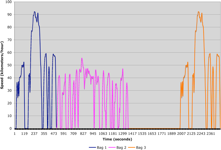
The portion of the FTP pattern in 6.2.2-5 that is considered the LA4 pattern is colored pink. This includes emissions collected in Bag 1 or Bag 3 followed by Bag 2 of the FTP cycle. A ‘cold start trip, or cold LA4, is using Bags 1 and 2, and a ‘hot’ LA4, or ‘hot start trip’ uses Bag 3 instead of Bag 1. The distance covered in Bag 1/3 is 3.59 miles and 3.91 miles for Bag 2. The overall weighted emissions of an FTP are reported in grams/mile and can be calculated as .206*Bag1 emissions/3.59 miles + .521*Bag 2 emissions/3.91 + .273*Bag 3 emissions/3.59 miles.
Since the introduction of Global Positioning Satellite Units (GPS), which can collect second by second data quickly and accurately over long periods of time, many areas are using this data to collect and design a set of representative cycles for all of the different road types and congestion situations in the areas. These are sometimes called ‘facility cycles’ by the US EPA, which has 14 different cycles to represent the speed and acceleration profile at different roadway types and levels of congestion. This is used in the newest version of the MOBILE model. California uses a set of Unified Correction Cycles to model similar effects of roadway conditions. Germany has developed a comprehensive set of 43 driving cycles from a large GPS data set.
All of the cycles developed in each area are different, however, they all are velocity profiles and they are all classified by road type. At a minimum, roadways are often classified into one of four classes:
"1. Residential Streets - Roads that carry vehicles into and through residential areas, typically exhibiting lower speeds, many stops, and/or speed bumps."
2. Arterials - Roads that connect one part of a city to another, usually with slow to moderate speeds, with some stops or stop lights.
3. Highways- Roads that connect one city to another city or cross a city, with minimal stops.
4. Freeways - Limited access roads for moving from city to city or across a city, usually with on and off-ramps and no stops.
Freeways are highly developed in the United States and parts of Europe. They are less prevalent in many developing countries. It is common to combine highways and freeways into a single road category usually referred to as Highways resulting in three categories of roadways. It also goes, almost without saying, that some residential streets operate similarly to arterials and some arterials operate similarly to highways. However, for the sake of simplicity, the three to four categories of streets as outlined above are normally used to carry out air pollution and other road related studies in urban areas.
Based on studies carried out by ISSRC in various countries around the world, the dominant number of road kilometers in an urban area is on residential streets by a three to one margin compared to arterials and highways combined. Arterials are second in total length, and highways are the least. ISSRC has also cataloged vehicle driving patterns by road type and by hour of the day for a number of cities around the world in order to understand how driving varies by road class and to improve emission estimates.
6.2.2.4 Moving beyond Static Velocity & Acceleration Profiles to Estimate Emissions Effects of Vehicle Operation
Many of the methods described in previous paragraphs use a type of velocity profile correction to model the effect of vehicle operations on emissions. This means that if a modeler would like to estimate emissions on the freeway, he would measure (or assume) the average velocity on that roadway and select a cycle that has similar average velocities. However, there are inherent problems with this approach, since the average velocity of a cycle is a poor indicator of emissions over that cycle. A much better indicator is combining velocity with acceleration. This is done in a modal emissions approach that defines an emission rate or correction for various operating modes, such as idle, cruise, and acceleration and deceleration. However, this is still a ‘static’ approach and cannot take into consideration road grade, use of accessory power consumption or other time-dependent factors such as catalyst loading or delayed responses.
Even more recently, a different, more accurate method of estimating emissions from vehicles is being used in the US and Europe that does not rely on a specific velocity-based cycle, rather a set of operational conditions that can be described using vehicle specific power. This method of characterizing vehicle operation can take into consideration dynamic factors and other considerations that have an effect on fuel use and emissions output, such as road grade, using the air conditioner, etc.
6.2.2.5 Fuel Quality
As discussed in subsection 6.2.1, fuel type and quality can have significant impacts on vehicle emissions. The most important considerations related to fuel quality are summarized in table 6.2.2-6. Most emission factors for vehicles are based on standard fuels. When estimating emissions, adjustments should be made for the cases where fuel quality results in more or less emissions than the standard fuels. Most vehicle emission models allow for some adjustment to the model calculations based on fuel quality.
6.2.2.6 Start Emissions and Start Patterns
In order to make a vehicle start easier, more fuel is normally supplied to the engine. This causes the air/fuel mixture to become richer which makes the vehicle start easier, especially in cold weather. However, this procedure also increases the emissions from the vehicle until the air/fuel ratio is returned to the normal rate. Vehicles manufactured in the United States before 1960 often had a manual adjustment for the air/fuel mixture called a “choke”, which would richen the mixture when pulled and then was manually shut off once the vehicle was warmed up. Modern vehicles handle this adjustment automatically so that the driver is normally unaware that such an adjustment is taking place. These extra emissions that occur as the vehicle is started and warmed up are referred to as start emissions. With the addition of catalysts to vehicles, the emissions associated with a vehicle start compared to normal operations increased further since the catalyst is ineffective until it is warmed up. Thus, an important emissions concern with respect to vehicles is the start emissions associated with the vehicle. Catalyst controlled vehicles tend to have relatively larger start emissions compared to non-catalyst controlled vehicles.
Start emissions are defined as the emissions in excess of normal warm vehicle emissions that occur during the first few minutes of vehicle operation. A vehicle that has been operated so that the engine and catalyst are at least somewhat warm will have less start emissions than a vehicle that has sat for a long time and the engine and catalyst are at ambient temperatures. Thus, there are different start emissions associated with a vehicle that has stopped for only a few minutes and then re-started compared to a vehicle that has not operated for 12 or more hours. The time that a vehicle is not operated is referred to as the “soak” period. The start emissions then vary with the soak period from almost zero with a soak period of less than 15 minutes to the maximum amount after about twelve hours of non-operation soak.
In order to estimate start emissions associated with a single vehicle, one must determine how many times a vehicle is started each day and how long the vehicle has soaked before each start. This is called the vehicle start pattern. When evaluating emissions from a whole fleet of vehicles, then one must determine the start pattern for each vehicle and then add all of the start patterns to produce a single overall start pattern for the whole fleet. It is common to break the starts down by each hour of the day or at least by four hour time periods and to indicate the number of starts in each time period and the distribution of the soak patterns for that time period. Start patterns are discussed further in 6.2.8, “Determination of Start-Up Patterns of On-Road Vehicles.”
It is not unusual for vehicle emission factors to include some start emissions built into the emission factor. Of course, to do this, assumptions must be made about the typical soak time before a start and the number of starts per day. These factors cannot be used to get a reliable estimate of the start emission variation by the hour of the day.
6.2.2.7 Other Operational Considerations
Altitude, temperature, and humidity can also have some impact on emissions, but the impacts of temperature and humidity are typically small except in the case of extreme temperatures and are thus often ignored. Altitude is an important factor especially in the case of carbureted vehicles. Carbureted vehicles do not automatically compensate for altitude. The air/fuel mixture in the engine becomes rich due to the reduced density of the air and CO and HC emissions increase. Modern fuel injected vehicles with computer controls and an oxygen sensor are designed to adjust for altitude and so the altitude impacts are much lower for these vehicles than in the case of carbureted vehicles.
6.2.2.8 Summary of Fleet Information and Vehicle Operational Data
In summary, the distribution of technologies or model years must be established to determine the fleet information, which can involve up to 1440 categories or more. Then, the vehicle operation, including the speed, acceleration, and other operational conditions of the traffic on each road type, the number and conditions of starting, and the diurnal activity, must be established. Finally, temperatures, altitude, humidity, and fuel quality can be factored into the calculation to improve estimates. With this information, an emission factor as a function of vehicle type and vehicle operation must be established for the fleet in question. These parameters can be combined in order to reach the final goal of determining the emissions from the on-road vehicle fleet.