Air Quality Modeling
7.3 Atmospheric Reaction Modeling
7.3.2 Three Dimensional Eulerian Grid Models
7.3.2.1 Theoretical Basis
The starting point of atmospheric chemical transport models is the mass balance equation for a chemical species i,
where (x, t) is the concentration of i as a function of location x and time t, u (x. t) is the velocity vector (
 ,
, ,
, ) ,
) ,  is the chemical generation term for i, and
  (x, t) and
  (x, t) are its emission and removal fluxes, respectively. This equation leads directly to the atmospheric diffusion equation by splitting the atmospheric transport term into an advection and turbulent transport contribution,
where(x,y,z,t), (x,y,z,t), and (x,y,z,t) are the x, y and z components of the wind velocity,  (x,y,z,t),
  (x,y,z,t), and
  (x,y,z,t) the corresponding eddy diffusivities. The turbulent fluctuations
  and
and  of the velocity and concentration fields relative to their average values u and have been approximated using the K theory (or mixing length or gradient transport theory) in equation 7.3.2-3 by
Equation 7.3.2-3 is the simplest solution to the closure problem and is currently used in the majority of chemical transport models. Higher-order closure approximations have been developed but are computationally expensive. Recently, some formulations have shown promise of becoming computationally competitive with the commonly employed K theory (Pai and Tsang, 1993).
7.3.2.2 Coordinate System-Uneven Terrain
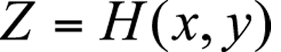
In our discussion so far we have implicitly assumed that the terrain is flat. Obviously, this is rarely the case. For example, severe air pollution problems often occur in airsheds that are at least partially bounded by mountains that restrict air movement. The surface of the Earth can be characterized by is topography,
The upper boundary of the modeling domain can be characterized by the mixing height (x,y,z,t) or an appropriately chosen constant height
  . The presence of topographic relief complicates the numerical solution of the atmospheric diffusion equation. Instead of using the actual height of a site (i. e., measured using sea level as a reference height) one usually transforms the domain into one of simpler geometry (7.3.2-1).This can be accomplished by a mapping that transforms points (x,y,z) from the physical domain to points (
 ) of the computational domain. The terrain-following coordinate transformation is commonly used, where
that scales the vertical extent of the modeling domain into a new domain that varies from 0 to 1.
7.3.2.3 Initial Conditions
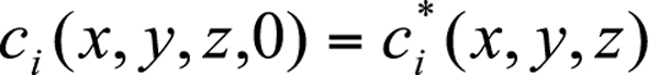
The solution of the full atmospheric diffusion equation requires the specification of the initial concentration field of all species
A typical modeling domain at the urban or global scales contains on the order of 103 computational cells, and as a result one needs to specify the concentrations of all simulated species at all these points. There are practically never sufficient measurements (especially for the upper-lever computational cells), so one needs to extrapolate from the few available data to the rest of the modeling domain. Use of an inaccurate concentration field may introduce significant errors during the early part of the simulation. Initially, the model prediction is equal to , the specified initial concentration, and will obviously be only as good at the specified value. As the simulation proceeds the initial condition term decays exponentially, while those due to emissions and advection increase in relative magnitude. Even if the specified initial conditions contain gross errors, their effect is eventually lost and the solution is dominated by the emissions
  and the boundary conditions
  . It is therefore common practice to start atmospheric simulations some period of time before that which is actually of interest. At the end of this “start-up” period the model should have established concentration fields that do not seriously reflect the initial conditions and the actual simulation and comparison with observations may commence. The start-up period for any atmospheric chemical transport model is determined by the residence time
  of an air parcel in the modeling domain.
7.3.2.4 Boundary Conditions
The atmospheric diffusion equation in three dimensions requires side boundary conditions, two for each of the x, y and z directions. The only exception are global scale models simulating the whole Earth’s atmosphere. One usually specifies the concentrations at the side boundaries of the modeling domain as a function of time,
Unfortunately, species concentration fields are practically never known at all points of the boundary of a modeling domain. Unlike initial conditions, boundary conditions, especially at the upwind boundaries, continue to affect predictions throughout the simulation. The simple box model solution once more provides valuable insights as represents the corresponding boundary conditions. After the start-up period the solution is the sum of the emission term and a term proportional to the concentration at the boundary. If  , errors it will have a small effect on the model predictions, which will be dominated by emissions. Therefore one should try to place the limits of the modeling domain in relatively clean areas (low ), where boundary conditions are relatively well known and have a relatively small effect on model predictions. A rule of thumb is to try to include all sources that have any effect on the air quality of a given region inside the modeling domain. If this cannot be done because of computational constraints, then the source effect has to be included implicitly in the boundary conditions. Uncertainty in urban air pollution model predictions as a result of uncertain side boundary conditions may be reduced by use of larger scale models (e. g., regional models) to provide the boundary conditions to the urban scale model. This technique is called nesting (the urban scale model is “nested” inside the regional scale model).
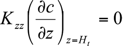
Treatment of upper and lower boundary conditions is different from that of the side conditions. One usually chooses a total reflection condition at the upper boundary of the computational domain (e. g., the top of the planetary boundary layer)
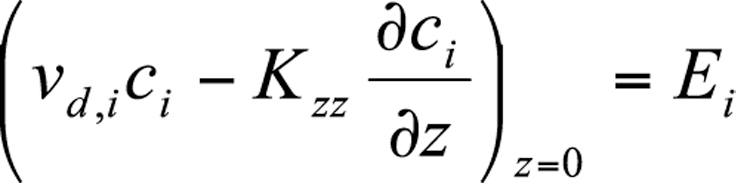
The boundary condition used at Earth’s surface accounts for surface sources and sinks of material,
where is the deposition velocity and is the ground-level emission rate of the species. Note that ground-level emissions can be included either as part of the z=0 boundary condition or directly in the differential equation as a source term in the ground-level cells.
The starting point of atmospheric chemical transport models is the mass balance equation for a chemical species i,
where
(x, t) is the concentration of i as a function of location x and time t, u (x. t) is the velocity vector (,,) , is the chemical generation term for i, and (x, t) and (x, t) are its emission and removal fluxes, respectively. This equation leads directly to the atmospheric diffusion equation by splitting the atmospheric transport term into an advection and turbulent transport contribution,
where
(x,y,z,t), (x,y,z,t), and (x,y,z,t) are the x, y and z components of the wind velocity, (x,y,z,t), (x,y,z,t), and (x,y,z,t) the corresponding eddy diffusivities. The turbulent fluctuations and of the velocity and concentration fields relative to their average values u and have been approximated using the K theory (or mixing length or gradient transport theory) in equation 7.3.2-3 by
Equation 7.3.2-3 is the simplest solution to the closure problem and is currently used in the majority of chemical transport models. Higher-order closure approximations have been developed but are computationally expensive. Recently, some formulations have shown promise of becoming computationally competitive with the commonly employed K theory (Pai and Tsang, 1993).
7.3.2.2 Coordinate System-Uneven Terrain
In our discussion so far we have implicitly assumed that the terrain is flat. Obviously, this is rarely the case. For example, severe air pollution problems often occur in airsheds that are at least partially bounded by mountains that restrict air movement. The surface of the Earth can be characterized by is topography,
The upper boundary of the modeling domain can be characterized by the mixing height
(x,y,z,t) or an appropriately chosen constant height . The presence of topographic relief complicates the numerical solution of the atmospheric diffusion equation. Instead of using the actual height of a site (i. e., measured using sea level as a reference height) one usually transforms the domain into one of simpler geometry (7.3.2-1).This can be accomplished by a mapping that transforms points (x,y,z) from the physical domain to points () of the computational domain. The terrain-following coordinate transformation is commonly used, where
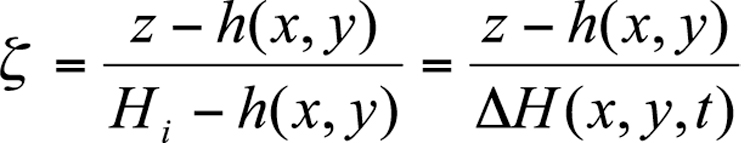
that scales the vertical extent of the modeling domain into a new domain
that varies from 0 to 1.

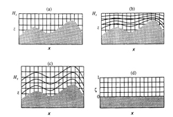
7.3.2-6 Coordinate Transformation for Uneven Terrain. (a) Two-dimensional terrain in x-z space. (b) Same as (a) but with contours of constant superimposed. (c) Same as (a) but with contours of constant  superimposed. (d) Two-dimensional terrain in x- computational space. The terrain is indicated by the shaded region
superimposed. (c) Same as (a) but with contours of constant superimposed. (d) Two-dimensional terrain in x- computational space. The terrain is indicated by the shaded region7.3.2.3 Initial Conditions
The solution of the full atmospheric diffusion equation requires the specification of the initial concentration field of all species
A typical modeling domain at the urban or global scales contains on the order of 103 computational cells, and as a result one needs to specify the concentrations of all simulated species at all these points. There are practically never sufficient measurements (especially for the upper-lever computational cells), so one needs to extrapolate from the few available data to the rest of the modeling domain. Use of an inaccurate concentration field may introduce significant errors during the early part of the simulation. Initially, the model prediction is equal to
 , the specified initial concentration, and will obviously be only as good at the specified value. As the simulation proceeds the initial condition term decays exponentially, while those due to emissions and advection increase in relative magnitude. Even if the specified initial conditions contain gross errors, their effect is eventually lost and the solution is dominated by the emissions and the boundary conditions . It is therefore common practice to start atmospheric simulations some period of time before that which is actually of interest. At the end of this “start-up” period the model should have established concentration fields that do not seriously reflect the initial conditions and the actual simulation and comparison with observations may commence. The start-up period for any atmospheric chemical transport model is determined by the residence time of an air parcel in the modeling domain.
7.3.2.4 Boundary Conditions
The atmospheric diffusion equation in three dimensions requires side boundary conditions, two for each of the x, y and z directions. The only exception are global scale models simulating the whole Earth’s atmosphere. One usually specifies the concentrations at the side boundaries of the modeling domain as a function of time,
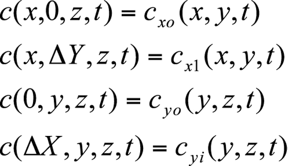
Unfortunately, species concentration fields are practically never known at all points of the boundary of a modeling domain. Unlike initial conditions, boundary conditions, especially at the upwind boundaries, continue to affect predictions throughout the simulation. The simple box model solution once more provides valuable insights as
represents the corresponding boundary conditions. After the start-up period the solution is the sum of the emission term and a term proportional to the concentration at the boundary. If , errors it will have a small effect on the model predictions, which will be dominated by emissions. Therefore one should try to place the limits of the modeling domain in relatively clean areas (low ), where boundary conditions are relatively well known and have a relatively small effect on model predictions. A rule of thumb is to try to include all sources that have any effect on the air quality of a given region inside the modeling domain. If this cannot be done because of computational constraints, then the source effect has to be included implicitly in the boundary conditions. Uncertainty in urban air pollution model predictions as a result of uncertain side boundary conditions may be reduced by use of larger scale models (e. g., regional models) to provide the boundary conditions to the urban scale model. This technique is called nesting (the urban scale model is “nested” inside the regional scale model).
Treatment of upper and lower boundary conditions is different from that of the side conditions. One usually chooses a total reflection condition at the upper boundary of the computational domain (e. g., the top of the planetary boundary layer)
The boundary condition used at Earth’s surface accounts for surface sources and sinks of material,
where
is the deposition velocity and is the ground-level emission rate of the species. Note that ground-level emissions can be included either as part of the z=0 boundary condition or directly in the differential equation as a source term in the ground-level cells.