Air Quality Modeling
7.2 Dispersion Modeling
7.2.1 Gaussian Dispersion
7.2.1.1 Theoretical Basis
Gaussian diffusion models are extensively used in assessing the impacts of existing and proposed sources of air pollution on local and urban air quality, particularly for regulatory applications. The history of Gaussian diffusion modeling goes back to the early 1920s when foundations of gradient transport and statistical theories of diffusion were laid. Earlier, temperature distributions in certain heat conduction problems were shown to be Gaussian, as were the concentration distributions in problems of molecular (Brownian) diffusion. In his classical paper on scattering of smoke in a turbulent atmosphere, Roberts (1923) obtained the solutions to the mean diffusion equation with constant-eddy diffusivities for different source configurations. His solutions showed Gaussian distributions in ensemble-averaged smoke puffs from an instantaneous point source. Gaussian concentration distributions were also derived in plumes from continuous point and line sources under certain simplifying assumptions (equivalent to the slender-plume approximation). Although Roberts (1923) did not put his solutions in the standard Gaussian forms, using ,
,  , and so on, he provided the original theoretical basis for what came to be known as Gaussian diffusion models. A stronger theoretical basis, without recourse to the questionable gradient transport hypothesis, was later provided by the statistical theories and random-walk models of particle dispersion in homogeneous turbulent flows.
Theoretical basis for Gaussian diffusion models is limited to idealized uniform flows with homogeneous turbulence. For continuous point and line sources, mean wind speed is also required to be larger than the standard deviations of turbulent velocity fluctuations, so that the upstream or longitudinal diffusion can be neglected. Mean winds and turbulence encountered in the atmosphere, particularly in the PBL, rarely satisfy the above simplifying assumptions of the theory. Frequently, one encounters significant wind shears, in-homogeneities of turbulence, and weak winds to make the theoretical basis of Gaussian diffusion modeling somewhat tenuous, if not totally invalid.
7.2.1.2 Other Justifications
The primary justification for the use of Gaussian dif-fusion models in regulatory applications comes from their evaluation and validation against experimental diffusion data. Much of the data used for this purpose are, however, limited to near-field or maximum ground level concentrations and the meteorological and source parameters that are used as input to Gaussian models. Since the regulatory emphasis is also on near-source maximum, the limited evaluation and validation of models against observed may be well justified. Other reasons for using Gaussian diffusion models in regulatory applications are:
1. They are analytical and conceptually appealing.
2. They are consistent with the random nature of turbulence.
3. They are computationally cheaper to use.
4. They have acquired an offcial "blessed" status in reg-ulatory guidelines (U.S. Environmental Protection Agency, 1986, 1996).
7.2.1.3 Other Justifications
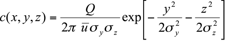
The cornerstone of most dispersion calculations in regulatory applications is the Gaussian plume formula for a continuous point source in a uniform flow with homogeneous turbulence:
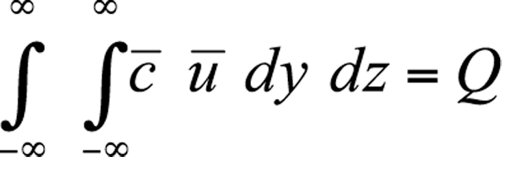
Here Q is the source strength or emission rate, is the mean transport velocity across the plume, and and are the Gaussian plume dispersion parameters. Equation 7.2.1-1 can be derived simply from the assumption of Gaussian concentration distributions in y and z directions at any cross section in the plume downwind of the source, and the integral mass-conservation condition.
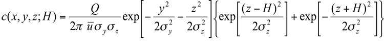
Since most point sources of pollution in the atmosphere are located at or near the earth's surface (e.g., vents, valves, stacks, and chimneys), it is necessary to account for the presence of the ground surface. Assuming perfectly reflecting surface as the most conservative boundary condition, addition of an "image" source yields the following reflected-Gaussian formula for a surface or an elevated release:
where H is the effective height of release above the ground. Note that equation 7.2.1-3 satisfies the mass-conservation condition equation 7.2.1-2 with the lower limit on z changed from to 0. Following D.B. Turner (1994), Equation 7.2.1-3 can be thought of as a product of four factors:
1. The emission factor, Q, which indicates that concentration at any point is directly proportional to the emission rate or the source strength.
2. The inverse mean wind factor, , which indicates that concentrations are inversely proportional to mean wind speed.
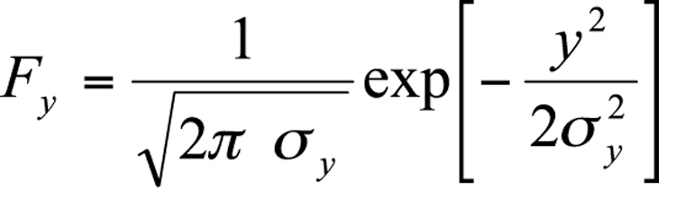
3. The cross-wind dispersion factor
which indicates that along the y axis, concentration is normally distributed, with the maximum value at the plume centerline which is inversely proportional to the lateral dispersion parameter,.
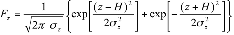
4. The vertical dispersion factor
which indicates that, in the vertical direction (z axis), concentration distribution is given by the sum of the Gaussian distributions due to real and image sources, respectively, and concentration is inversely proportional to the vertical dispersion parameter, .
.
7.2.1.4 Assumptions and Approximations in Gaussian Plume Model
Many assumptions and approximations are implied in the Gaussian plume model. Some of the important assumptions are (Lyons and Scott, 1990):
1. Continuous emission from the source at a constant rate, at least for a time equal to or greater than the time of travel to the location (receptor) of interest. The plume diffusion formulae assume that release and sampling times are long compared with the travel time to receptor, so that the material is spread out in the form of a steady plume between the source and the farthest receptor. A shorter release will result in an elongated puff with a time-dependent concentration field.
2. Steady-state flow and constant meteorological conditions, at least over the time of transport (travel) from the source to the farthest receptor. This assumption may not be valid during rapidly changing meteorological conditions, such as during the passage of a front or a storm and also during the morning and evening transition periods.
3. Conservation of mass in the plume. The continuity equation satisfied by the Gaussian plume formula (7.2.1-4) is a mathematical expression of the condition that the mass flow rate through any plume cross section is equal to the source emission rate. This implies that none of the material is removed through chemical reaction, gravitational settling, or deposition at the surface. All the material reaching the surface through turbulent dif-fusion is reflected back and none is absorbed there.
4. Gaussian or reflected Gaussian distribution of mean concentration in the lateral (cross-wind) and vertical directions at any downwind location in the plume. The assumption of Gaussian distribution in the vertical direction is somewhat questionable, but does not appear to affect adversely the model predicted ground-level concentrations.
5. A constant mean transport wind in the horizontal (x-y) plane. This implies horizontal homogeneity of flow and the underlying surface and becomes invalid over a complex terrain.
6. No wind shear in the vertical. This assumption is implicit in the constant mean transport velocity in the Gaussian plume formulae. In practice, is often taken as the wind speed at 10 m height for near-surface sources (H**10 m) and the wind speed at the effective release height for elevated sources. The variation of wind speed with height can also be considered in more accurately estimating the effective transport velocity, but this requires the knowledge of vertical concentration distribution in the plume at each receptor location. The variation of wind direction with height is ignored, although its effect on the lateral plume spread and concentration field can be considered superficially through an appropriate parameterization of .
7. Strong enough winds to make turbulent diffusion in the direction of flow negligible in comparison with mean transport. This assumption, also known as the slender-plume approximation, which is implicit in the Gaussian plume model, generally becomes invalid very close to the source where material diffuses up-wind of the source due to longitudinal velocity fluctuations. The assumption becomes invalid farther and farther away from the source as mean wind becomes weaker and vanishes entirely (e.g., under extremely stable and free convection conditions).
Additional assumptions are introduced in the specification of meteorological and dispersion parameters in the Gaussian plume model. These will be discussed in the next section.
7.2.1.5 Limitations of Gaussian Diffusion Models
Limitations of most operational air quality and dispersion models arise from the simplifying assumptions implied in their formulation, simplified physics, and parameterization of complex turbulence and diffusion processes in these models. In particular, Gaussian diffusion models have limited applicability for relatively flat and homogeneous surfaces, reasonably steady and moderate to strong winds, moderately stable and unstable conditions, neutrally buoyant or slightly buoy-ant emissions, and relatively short distances (**50 km) from simple source configurations. Even under these idealized conditions, Gaussian diffusion models have large uncertainties due to natural variability and simplified model physics. Significant deviations from the idealized conditions introduce further limitations on the validity of such models, because model uncertain-ties might become too large to be acceptable. Gifford (1976) considered these as exceptional conditions, which include near-calm, extremely stable, and convective conditions; very rough (e.g., cities and forests) or very smooth (e.g., water) surfaces for which suggested diffusion parameterization may not be applicable; irregular and rugged terrain; and the presence of obstacles (e.g., hills and buildings) to the flow. To these one might add highly buoyant and dense gas emissions, stack downwash, and emissions of particulate matter and highly reactive gases. More sophisticated numerical models must be used to simulate and predict dispersion in these complex flow conditions.
Gaussian diffusion models are extensively used in assessing the impacts of existing and proposed sources of air pollution on local and urban air quality, particularly for regulatory applications. The history of Gaussian diffusion modeling goes back to the early 1920s when foundations of gradient transport and statistical theories of diffusion were laid. Earlier, temperature distributions in certain heat conduction problems were shown to be Gaussian, as were the concentration distributions in problems of molecular (Brownian) diffusion. In his classical paper on scattering of smoke in a turbulent atmosphere, Roberts (1923) obtained the solutions to the mean diffusion equation with constant-eddy diffusivities for different source configurations. His solutions showed Gaussian distributions in ensemble-averaged smoke puffs from an instantaneous point source. Gaussian concentration distributions were also derived in plumes from continuous point and line sources under certain simplifying assumptions (equivalent to the slender-plume approximation). Although Roberts (1923) did not put his solutions in the standard Gaussian forms, using
, , and so on, he provided the original theoretical basis for what came to be known as Gaussian diffusion models. A stronger theoretical basis, without recourse to the questionable gradient transport hypothesis, was later provided by the statistical theories and random-walk models of particle dispersion in homogeneous turbulent flows.
Theoretical basis for Gaussian diffusion models is limited to idealized uniform flows with homogeneous turbulence. For continuous point and line sources, mean wind speed is also required to be larger than the standard deviations of turbulent velocity fluctuations, so that the upstream or longitudinal diffusion can be neglected. Mean winds and turbulence encountered in the atmosphere, particularly in the PBL, rarely satisfy the above simplifying assumptions of the theory. Frequently, one encounters significant wind shears, in-homogeneities of turbulence, and weak winds to make the theoretical basis of Gaussian diffusion modeling somewhat tenuous, if not totally invalid.
7.2.1.2 Other Justifications
The primary justification for the use of Gaussian dif-fusion models in regulatory applications comes from their evaluation and validation against experimental diffusion data. Much of the data used for this purpose are, however, limited to near-field or maximum ground level concentrations and the meteorological and source parameters that are used as input to Gaussian models. Since the regulatory emphasis is also on near-source maximum, the limited evaluation and validation of models against observed may be well justified. Other reasons for using Gaussian diffusion models in regulatory applications are:
1. They are analytical and conceptually appealing.
2. They are consistent with the random nature of turbulence.
3. They are computationally cheaper to use.
4. They have acquired an offcial "blessed" status in reg-ulatory guidelines (U.S. Environmental Protection Agency, 1986, 1996).
7.2.1.3 Other Justifications
The cornerstone of most dispersion calculations in regulatory applications is the Gaussian plume formula for a continuous point source in a uniform flow with homogeneous turbulence:
Here Q is the source strength or emission rate,
is the mean transport velocity across the plume, and and are the Gaussian plume dispersion parameters. Equation 7.2.1-1 can be derived simply from the assumption of Gaussian concentration distributions in y and z directions at any cross section in the plume downwind of the source, and the integral mass-conservation condition.
Since most point sources of pollution in the atmosphere are located at or near the earth's surface (e.g., vents, valves, stacks, and chimneys), it is necessary to account for the presence of the ground surface. Assuming perfectly reflecting surface as the most conservative boundary condition, addition of an "image" source yields the following reflected-Gaussian formula for a surface or an elevated release:
where H is the effective height of release above the ground. Note that equation 7.2.1-3 satisfies the mass-conservation condition equation 7.2.1-2 with the lower limit on z changed from
to 0. Following D.B. Turner (1994), Equation 7.2.1-3 can be thought of as a product of four factors:
1. The emission factor, Q, which indicates that concentration at any point is directly proportional to the emission rate or the source strength.
2. The inverse mean wind factor,
, which indicates that concentrations are inversely proportional to mean wind speed.
3. The cross-wind dispersion factor
which indicates that along the y axis, concentration is normally distributed, with the maximum value at the plume centerline which is inversely proportional to the lateral dispersion parameter,
.
4. The vertical dispersion factor
which indicates that, in the vertical direction (z axis), concentration distribution is given by the sum of the Gaussian distributions due to real and image sources, respectively, and concentration is inversely proportional to the vertical dispersion parameter,
.
7.2.1.4 Assumptions and Approximations in Gaussian Plume Model
Many assumptions and approximations are implied in the Gaussian plume model. Some of the important assumptions are (Lyons and Scott, 1990):
1. Continuous emission from the source at a constant rate, at least for a time equal to or greater than the time of travel to the location (receptor) of interest. The plume diffusion formulae assume that release and sampling times are long compared with the travel time to receptor, so that the material is spread out in the form of a steady plume between the source and the farthest receptor. A shorter release will result in an elongated puff with a time-dependent concentration field.
2. Steady-state flow and constant meteorological conditions, at least over the time of transport (travel) from the source to the farthest receptor. This assumption may not be valid during rapidly changing meteorological conditions, such as during the passage of a front or a storm and also during the morning and evening transition periods.
3. Conservation of mass in the plume. The continuity equation satisfied by the Gaussian plume formula (7.2.1-4) is a mathematical expression of the condition that the mass flow rate through any plume cross section is equal to the source emission rate. This implies that none of the material is removed through chemical reaction, gravitational settling, or deposition at the surface. All the material reaching the surface through turbulent dif-fusion is reflected back and none is absorbed there.
4. Gaussian or reflected Gaussian distribution of mean concentration in the lateral (cross-wind) and vertical directions at any downwind location in the plume. The assumption of Gaussian distribution in the vertical direction is somewhat questionable, but does not appear to affect adversely the model predicted ground-level concentrations.
5. A constant mean transport wind in the horizontal (x-y) plane. This implies horizontal homogeneity of flow and the underlying surface and becomes invalid over a complex terrain.
6. No wind shear in the vertical. This assumption is implicit in the constant mean transport velocity
in the Gaussian plume formulae. In practice, is often taken as the wind speed at 10 m height for near-surface sources (H**10 m) and the wind speed at the effective release height for elevated sources. The variation of wind speed with height can also be considered in more accurately estimating the effective transport velocity, but this requires the knowledge of vertical concentration distribution in the plume at each receptor location. The variation of wind direction with height is ignored, although its effect on the lateral plume spread and concentration field can be considered superficially through an appropriate parameterization of .
7. Strong enough winds to make turbulent diffusion in the direction of flow negligible in comparison with mean transport. This assumption, also known as the slender-plume approximation, which is implicit in the Gaussian plume model, generally becomes invalid very close to the source where material diffuses up-wind of the source due to longitudinal velocity fluctuations. The assumption becomes invalid farther and farther away from the source as mean wind becomes weaker and vanishes entirely (e.g., under extremely stable and free convection conditions).
Additional assumptions are introduced in the specification of meteorological and dispersion parameters in the Gaussian plume model. These will be discussed in the next section.
7.2.1.5 Limitations of Gaussian Diffusion Models
Limitations of most operational air quality and dispersion models arise from the simplifying assumptions implied in their formulation, simplified physics, and parameterization of complex turbulence and diffusion processes in these models. In particular, Gaussian diffusion models have limited applicability for relatively flat and homogeneous surfaces, reasonably steady and moderate to strong winds, moderately stable and unstable conditions, neutrally buoyant or slightly buoy-ant emissions, and relatively short distances (**50 km) from simple source configurations. Even under these idealized conditions, Gaussian diffusion models have large uncertainties due to natural variability and simplified model physics. Significant deviations from the idealized conditions introduce further limitations on the validity of such models, because model uncertain-ties might become too large to be acceptable. Gifford (1976) considered these as exceptional conditions, which include near-calm, extremely stable, and convective conditions; very rough (e.g., cities and forests) or very smooth (e.g., water) surfaces for which suggested diffusion parameterization may not be applicable; irregular and rugged terrain; and the presence of obstacles (e.g., hills and buildings) to the flow. To these one might add highly buoyant and dense gas emissions, stack downwash, and emissions of particulate matter and highly reactive gases. More sophisticated numerical models must be used to simulate and predict dispersion in these complex flow conditions.