Air Quality Modeling
7.1 Overview of Air Quality Modeling
7.1.4 The Classification of Air Quality Models
7.1.4.1 Introduction
Atmospheric models can be divided, broadly speaking, into two types: physical and mathematical. Physical models are sometimes used to simulate atmospheric processes by means of a small-scale representation of the actual system, for example, a small-scale replica of an urban area or portion thereof in a wind tunnel. Problems associated with properly duplicating the actual scales of atmospheric motion make physical models of this variety of limited usefulness. We henceforth focus our attention on mathematical models and the term model will refer strictly to mathematical models.
Mathematical models of atmospheric behavior can broadly be classified into two types:
1. Models based on the fundamental description of atmospheric physical and chemical processes.
2. Models based on statistical analysis of data.
Most regions contain a number of monitoring operated by governmental authorities at which l hour to daily average concentration levels are measured and reported. A great deal of information is potentially available in these enormous databases, and statistical analysis of such data can provide valuable insights. An example of how such data can be used is a simple forecast model, where, for a certain region, concentration levels in the next few hours are given as a statistical function of current concentrations and other variables from correlations among past measurements and concentration trends. Statistical models take advantage of the available databases and are relatively simple to apply. However, their reliance on past data is also their major weakness, because these models do not explicitly describe causal relationships, they cannot be reliably extrapolated beyond the bounds of the data from which they were derived. As a result, statistically based models are not ideally suited to the task of predicting the impact of significant changes in emissions. Models based on fundamental description of atmospheric physics and chemistry are the subjects of this chapter.
7.1.4.2 Lagrangian and Eulerian Models
A wide variety of atmospheric models have been proposed and used. Some of these simulate changes in the chemical composition of a given air parcel as it is advected in the atmosphere (Lagrangian models), while others describe the concentrations in an array of fixed computational cells (Eulerian models).
A Lagrangian modeling modeling framework is one that moves with the local wind so that there is no mass exchange between the air parcel and its surroundings, with the exception of species emissions that are allowed to enter the parcel through its base. The air Parcel moves continously, so the model actually simulates concentrations at different locations at different times. On the contrary, an Eulerian modeling framework remains fixed in space. Species enter and leave each cell through its walls, and the model simulates the species concentrations at all locations as a function of time.
7.1.4.3 Spatial and Temporal Scale
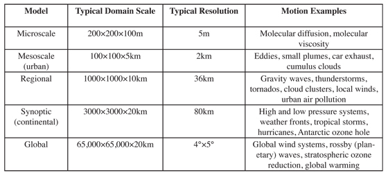
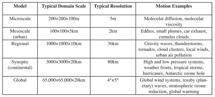
The domain of an atmospheric model that is, the area that is simulated varies from a few hundred meters to thousands of kilometers (see table 7.1.4-1) with different motions meteorology or phenomena occurring on each scale. The computational domain usually consists of an array of computational cells, each having a uniform chemical composition. The size of these cells, that is, the volume over which the predicted concentrations are averaged, determines the spatial resolution of the model. Variation of concentrations at scales smaller than the model resolution cannot easily be resolved. For example, concentration variations over the Los Angeles Basin cannot be described by a synoptic scale model that treats the entire area as one computational cell of uniform chemical composition.
Urban air pollution studies are simulated over a micro- to mesoscale domain, regional acid deposition is simulated over a meso-to synoptic scale domain, and global climate change studies are simulated over a global scale domain. Meteorological events occur over all scales. With respect to time, urban air pollution events are simulated over periods of hours to days, regional acid deposition events are simulated over periods of days to weeks, and climate change events are simulated over periods of months to hundreds of years and beyond.
7.1.4.4 Dimensionality
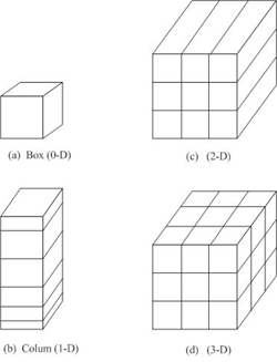 Atmospheric models are also characterized by their dimensionality. The simplest is the box model (zero-dimensional), where the atmospheric domain is represented by only one box (figure 7.1.4-2). In a box model concentrations are the same everywhere and therefore are functions of time only,
  (t). The next step in complexity are column models (one-dimensional) that assume that concentrations are functions of height and time, (z,t). The modeling domain consists of horizontally homogeneous layers. Two-dimensional models assume that species concentrations are uniform along one dimension and depend on the other two and time, for example, (x, z, t). Two-dimensional models have often been used in descriptions of global atmospheric chemistry, assuming that concentrations are functions of latitude and altitude but do not depend on longitude. Finally, three-dimensional models simulate the full concentration field (x, y, z, t). Obviously, both model complexity and accuracy increase with dimensionality. Governing equations of these models will be derived subsequently.
A zero-dimensional (0-D) model is a box model in which chemical and/or physical transformations occur. Gases and particles may enter or leave the box from any side. Since all material in the box is assumed to mix instantaneously, the concentration of each gas and particle is uniform throughout the box. A standard box model is fixed in space. A parcel model is a box model that moves through space along the direction of the wind. Emission enter the box at different locations and times. Because a parcel model moves in a Lagrangian sense, it is also called a Lagrangian trajectory model. Box models have been used to simulate photo chemical reactions that occur in smog chambers, fog production in a controlled environment, and chemical and physical interactions between aerosols and gases. Parcel models have been used to trace changes in an air parcel as it travels from ocean to land and through the polar ovrtex.
A one-dimensional (1-D) model is a set of adjacent box models, usually piled vertically. The advantages of a vertical 1-D model over a pure box model are that radiative transfer and vertical transport can be treated in a 1-D model. In a 1-Dmodel, gases and particles in each layer are permitted to attenuate solar radiation as it travels through the column. A unidirectional advection-diffusion equation can also be used to transport species in the column. The disadvantage of a 1-D model compared to a 2-D or 3-D model is that vertical velocities in a 1-Dmodel are crudely estimated, especially because they do not allow for horizontal variation in the wind. A 1-D model either ignores gas, particle, and potential temperature fluxes through horizontal boundaries or roughly parameterizes them. One-dimensional models have been used to simulate cloud formation, vertical profiles of gas concentrations, and vertical profiles of radiative fields.
A two-dimensional (2-D) model is a set of 1-D models connected side by side. 2-Dmodels can lie in the x-y, x-z,or y-z planes. Advantages of a 2-D over a 1-D model are that transport can be treated more realistically and a larger spatial region can be simulated in a 2-D model. 2-D models have been used to simulate transport, chemistry, and dynamics on a global scale (e.g.,Garcia et al.1992). A global 2-D model may stretch from the South to the North Pole and vertically. South-north and vertical winds in such a model are predicted or estimated from observations at each latitude and vertical layer. Zonally averaged winds (west-east winds, averaged over all longitudes for a given latitude and vertical layer) are needed in a 2-D global model. Such winds are found prognostically or diagnostically. Prognostic velocities are obtained by writing an equation of motion for the average west-east velocity at each latitude and altitude. Diagnostic velocities are obtained by writing prognostic equations for south-north and vertical velocities, then extracting the average zonal velocity from the continuity equation for air.
A three-dimensional (3-D) model is a set of horizontal 2-D models layered on top of one another. The advantage of a 3-D over a 2-D model is that dynamics and transport can be treated more realistically in a 3-D model. The disadvantage is that a 3-D model requires significantly more computer time and memory than does a 2-D model. In many cases, computer time is not a limitation. Studies of urban air pollution are readily carried out in 3-D, since simulation periods are generally only a few days. Computer-time limitations are most apparent for studies of global-scale problems that last months to years. Because 3-D models represent dynamical and transport processes better than do 0-, 1-, and 2-D models, 3-D models should be used when computer time requirements are not a hindrance.
Atmospheric models can be divided, broadly speaking, into two types: physical and mathematical. Physical models are sometimes used to simulate atmospheric processes by means of a small-scale representation of the actual system, for example, a small-scale replica of an urban area or portion thereof in a wind tunnel. Problems associated with properly duplicating the actual scales of atmospheric motion make physical models of this variety of limited usefulness. We henceforth focus our attention on mathematical models and the term model will refer strictly to mathematical models.
Mathematical models of atmospheric behavior can broadly be classified into two types:
1. Models based on the fundamental description of atmospheric physical and chemical processes.
2. Models based on statistical analysis of data.
Most regions contain a number of monitoring operated by governmental authorities at which l hour to daily average concentration levels are measured and reported. A great deal of information is potentially available in these enormous databases, and statistical analysis of such data can provide valuable insights. An example of how such data can be used is a simple forecast model, where, for a certain region, concentration levels in the next few hours are given as a statistical function of current concentrations and other variables from correlations among past measurements and concentration trends. Statistical models take advantage of the available databases and are relatively simple to apply. However, their reliance on past data is also their major weakness, because these models do not explicitly describe causal relationships, they cannot be reliably extrapolated beyond the bounds of the data from which they were derived. As a result, statistically based models are not ideally suited to the task of predicting the impact of significant changes in emissions. Models based on fundamental description of atmospheric physics and chemistry are the subjects of this chapter.
7.1.4.2 Lagrangian and Eulerian Models
A wide variety of atmospheric models have been proposed and used. Some of these simulate changes in the chemical composition of a given air parcel as it is advected in the atmosphere (Lagrangian models), while others describe the concentrations in an array of fixed computational cells (Eulerian models).
A Lagrangian modeling modeling framework is one that moves with the local wind so that there is no mass exchange between the air parcel and its surroundings, with the exception of species emissions that are allowed to enter the parcel through its base. The air Parcel moves continously, so the model actually simulates concentrations at different locations at different times. On the contrary, an Eulerian modeling framework remains fixed in space. Species enter and leave each cell through its walls, and the model simulates the species concentrations at all locations as a function of time.
7.1.4.3 Spatial and Temporal Scale
The domain of an atmospheric model that is, the area that is simulated varies from a few hundred meters to thousands of kilometers (see table 7.1.4-1) with different motions meteorology or phenomena occurring on each scale. The computational domain usually consists of an array of computational cells, each having a uniform chemical composition. The size of these cells, that is, the volume over which the predicted concentrations are averaged, determines the spatial resolution of the model. Variation of concentrations at scales smaller than the model resolution cannot easily be resolved. For example, concentration variations over the Los Angeles Basin cannot be described by a synoptic scale model that treats the entire area as one computational cell of uniform chemical composition.
Urban air pollution studies are simulated over a micro- to mesoscale domain, regional acid deposition is simulated over a meso-to synoptic scale domain, and global climate change studies are simulated over a global scale domain. Meteorological events occur over all scales. With respect to time, urban air pollution events are simulated over periods of hours to days, regional acid deposition events are simulated over periods of days to weeks, and climate change events are simulated over periods of months to hundreds of years and beyond.
7.1.4-1 Atmospheric Chemical Transport Models Defined According to Spatial Scale
7.1.4.4 Dimensionality
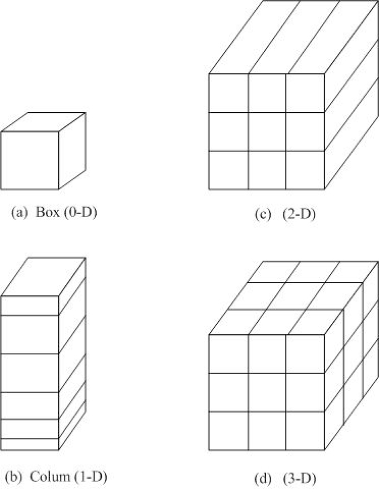
7.1.4-2 Schematic Depiction of (a) A Box Model (Zero-Dimensional), (b) A Column Model (One Dimensional) (c) A Two-Dimensional Model, and (d) A Three-Dimensional Model
(t). The next step in complexity are column models (one-dimensional) that assume that concentrations are functions of height and time, (z,t). The modeling domain consists of horizontally homogeneous layers. Two-dimensional models assume that species concentrations are uniform along one dimension and depend on the other two and time, for example, (x, z, t). Two-dimensional models have often been used in descriptions of global atmospheric chemistry, assuming that concentrations are functions of latitude and altitude but do not depend on longitude. Finally, three-dimensional models simulate the full concentration field (x, y, z, t). Obviously, both model complexity and accuracy increase with dimensionality. Governing equations of these models will be derived subsequently.
A zero-dimensional (0-D) model is a box model in which chemical and/or physical transformations occur. Gases and particles may enter or leave the box from any side. Since all material in the box is assumed to mix instantaneously, the concentration of each gas and particle is uniform throughout the box. A standard box model is fixed in space. A parcel model is a box model that moves through space along the direction of the wind. Emission enter the box at different locations and times. Because a parcel model moves in a Lagrangian sense, it is also called a Lagrangian trajectory model. Box models have been used to simulate photo chemical reactions that occur in smog chambers, fog production in a controlled environment, and chemical and physical interactions between aerosols and gases. Parcel models have been used to trace changes in an air parcel as it travels from ocean to land and through the polar ovrtex.
A one-dimensional (1-D) model is a set of adjacent box models, usually piled vertically. The advantages of a vertical 1-D model over a pure box model are that radiative transfer and vertical transport can be treated in a 1-D model. In a 1-Dmodel, gases and particles in each layer are permitted to attenuate solar radiation as it travels through the column. A unidirectional advection-diffusion equation can also be used to transport species in the column. The disadvantage of a 1-D model compared to a 2-D or 3-D model is that vertical velocities in a 1-Dmodel are crudely estimated, especially because they do not allow for horizontal variation in the wind. A 1-D model either ignores gas, particle, and potential temperature fluxes through horizontal boundaries or roughly parameterizes them. One-dimensional models have been used to simulate cloud formation, vertical profiles of gas concentrations, and vertical profiles of radiative fields.
A two-dimensional (2-D) model is a set of 1-D models connected side by side. 2-Dmodels can lie in the x-y, x-z,or y-z planes. Advantages of a 2-D over a 1-D model are that transport can be treated more realistically and a larger spatial region can be simulated in a 2-D model. 2-D models have been used to simulate transport, chemistry, and dynamics on a global scale (e.g.,Garcia et al.1992). A global 2-D model may stretch from the South to the North Pole and vertically. South-north and vertical winds in such a model are predicted or estimated from observations at each latitude and vertical layer. Zonally averaged winds (west-east winds, averaged over all longitudes for a given latitude and vertical layer) are needed in a 2-D global model. Such winds are found prognostically or diagnostically. Prognostic velocities are obtained by writing an equation of motion for the average west-east velocity at each latitude and altitude. Diagnostic velocities are obtained by writing prognostic equations for south-north and vertical velocities, then extracting the average zonal velocity from the continuity equation for air.
A three-dimensional (3-D) model is a set of horizontal 2-D models layered on top of one another. The advantage of a 3-D over a 2-D model is that dynamics and transport can be treated more realistically in a 3-D model. The disadvantage is that a 3-D model requires significantly more computer time and memory than does a 2-D model. In many cases, computer time is not a limitation. Studies of urban air pollution are readily carried out in 3-D, since simulation periods are generally only a few days. Computer-time limitations are most apparent for studies of global-scale problems that last months to years. Because 3-D models represent dynamical and transport processes better than do 0-, 1-, and 2-D models, 3-D models should be used when computer time requirements are not a hindrance.